Detailed description
Thermokinetics Software (TK)
Thermokinetics Software (TK) allows the determination of kinetic parameters (activation energy E and pre-exponential factor in Arrhenius equation A) of one-stage and complex, multistage overlapped reactions based on measurements performed by DSC, nano- and micro-DSC, isothermal and scanning calorimetry, DTA, TG and/or DTG, TG-MS, TG-FTIR and prediction of the reaction progress and thermal stability of materials under any temperature mode.
Advanced kinetic analysis, main features:
- Automatic baseline construction and use of the differential isoconversional method of Friedman (model free) for an advanced baseline optimization.
- Smoothing of data (Savitzky-Golay) and spikes correction.
- Differential isoconversional method of Friedman (model free).
- Integral isoconversional method of Ozawa-Flynn-Wall (model free).
- Standard procedure of ASTM A698.
- Calculations using kinetic models as e.g. n-th order approach (Fn), nucleation (Avrami-Erofeev, An, A2, A1.5), diffusion (parabolic law D1, Valesi D2, Jander D3, Brounshtein D4), movement of the phase boundary (shrinking core model, Rn, R1, R2), autocatalysis.
- Calculations using custom kinetic equation introduced by the user
- – e.g. dα/dt =1e10 * exp(-100000/8.314/(T+273.15)) * (1-α)
- – or dα/dt = A(α) * exp(-E(α)/8.314/(T+273.15)) * (1-α)
Prediction of the reaction progress and thermal stability of materials under any temperature mode:
- Isothermal and non-isothermal, stepwise.
- Modulated temperature or periodic temperature variations.
- Rapid temperature increase (temperature shock).
- Real atmospheric temperature profiles for investigating properties of e.g. low-temperature decomposed substances under different climates (yearly temperature profiles with daily minimal and maximal fluctuations. 50 default climates available).
- NATO norm STANAG 2895 temperature profile: Zones A1, A2, A3, B1, B2, B3, C0, C1, C2, C3, C4, M1, M2, M3.
- Customized temperature profiles: possibility to compare the reaction progress of substances at any temperature profile.
- Combination of mass loss TG and/or heat flow signal e.g. DSC/DTA and MS data for simultaneous comparison of the mass loss, heat flow and rate of evolution of volatile species at any temperature profile.
- Confidence interval of the prediction.
- Viewing data in form of overall conversion α (T(t)), or rate of the conversion dα/dt (T(t)) as a function of time or temperature.
- Viewing raw data as e.g. Q, dQ/dt, P, dP/dt, m, dm/dt.
- Extended features for High Sensitivity Isothermal Heat Flow Calorimetry (HFC): Ability to calculate the thermokinetic data from long-term isothermal HFC measurements for very precise lifetime prediction based on the initial reaction extent laying in the range of a few percent only.
Introduction
Application of thermokinetics for determination of materials’ behavior
The main goal of AKTS-Thermokinetics Software Package [1] is to facilitate the kinetic analysis of any type of thermoanalytical data (DSC, DTA, TGA, TG-MS or TG-FTIR, HFC) for the study of raw materials and products within the scope of research, development and quality. The main challenge is the prediction of the shelf life and the thermal stability of substances submitted to extended temperature ranges or such temperature conditions for which experimentation is difficult or impossible. These difficulties are prevalent at low temperatures (requiring a very long investigation time), as well as under specific temperature fluctuations. The goal of our advanced numerical approach is:
- A deeper insight into the reaction course of any material.
- Evaluation of the stability/reactivity from the data collected at the early stage of the decomposition.
Analysis Process
A full kinetic analysis of a solid state reaction has at least three major steps [1-7]
- (1) Experimental collection of data;
- (2) Computation of kinetic parameters using the data from step 1;
- (3) Prediction of the reaction progress for required temperature profiles applying calculated kinetic parameters.
The graph presented below depicts the evaluation of the kinetic parameters and prediction of the reaction course based on the data collected during DSC measurements. The workflow contains three major steps: (1) elaboration of the experimental data, (2) kinetic analysis and (3) the prediction of the reaction course under any temperature mode.
1. Baseline construction at least on two signals.
2. Click on ‘Bsl auto’ to construct automatically the baselines for the remaining signals.
3. Click on ‘Kinetics’ to apply the differential isoconversional analysis.
4. Ther are 2 methods for improving the baseline construction:
1) Manual adjustment of the baselines.
2) Optional: ‘OBsl’ = Optimize Baselines = Automatic adjustment of all baselines (one-two minutes).
5. Click on ‘Simulation’ to display the calculated reaction progress.
6. ‘Optimization’ of kinetic parameters for final adjustment of simulated signals.
7. ‘Prediction’ of the reaction rate and progress at any temperature profiles.
Fig. 1 – Application of DSC data for calculation of the reaction extent as a function of temperature, evaluation of kinetic parameters and simulation of the reaction progress at any temperature profile.
Elaboration of experimental data (STEP 1)
In this step the dependence of the reaction extent on time or temperature is evaluated from the experimental data. The knowledge of this dependence is the prerequisite of the further kinetic analysis. Below we illustrate the applied procedure using the DSC data for which the correct construction of the baseline is a crucial for the correctness of the kinetic calculations.
DSC experiments were performed in gold plated high pressure sealed crucibles at a heating rates of 0.5, 1, 2, 4 and 8 K/min (non-isothermal) with sample masses between 6.66 and 11.28 mg (AKTS recommends to use the high pressure sealed crucibles of TÜV SÜD Process Safety (Formerly: Swiss Institute for the Promotion of Safety and Security [8]). The measured data were subsequently exported in ASCII format for further thermokinetic interpretation with AKTS-Thermokinetics Software. Figures 2 show the DSC signals recorded at different heating rates.
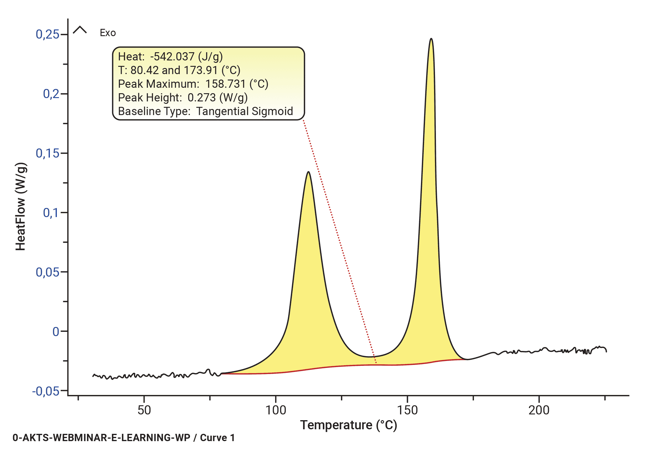
Fig. 2 – DSC curves of the examined material recorded at 0.5, 1, 2, 4 and 8 K/min (black curves: simulations of the reaction course based on kinetic parameters evaluated by differential isoconversional analysis).
The construction of the correct baseline is a crucial procedure in avoiding introduction of systematic errors during kinetic elaboration of the DSC/DTA data. Generally, the application of the straight-line form for the baseline is incorrect [9]. The recorded signal results not only from the heat of the reaction but is additionally affected by the change of the specific heat and its temperature dependence of the reactants and products during the progress of the reaction.
With
| symbol | name | units |
|---|---|---|
| B(t) | The baseline |  |
| S(t) | The differential signal | |
 | The reaction rate |  |
and the reaction progress α(t) [-] can be expressed as
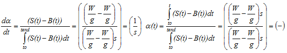
with
0 < α(t) < 1) and B(t) = (1- α(t))*(a1+b1*t) + α(t)*(a2+b2*t)
where
(a1+b1*t): Tangent at the beginning of the signal S(t)
(a2+b2*t): Tangent at the end of the signal S(t)
The most universal type, because of its correction possibilities, is the tangential area-proportional baseline. It is created at α(t) ![]() 0 and at α(t)
0 and at α(t) ![]() 1 by the appropriate tangents at the beginning or the end of the measured DSC signal. It allows compensation of not only changes in the value of Cp of the reactant and product, but also of changes in their temperature dependency. This type of baselines can be described by the following equation:
1 by the appropriate tangents at the beginning or the end of the measured DSC signal. It allows compensation of not only changes in the value of Cp of the reactant and product, but also of changes in their temperature dependency. This type of baselines can be described by the following equation:
B(t) = (1-α(t))*(a1+b1*t) + α(t)*(a2+b2*t)
with
(a1+b1*t): tangent at the beginning of the signal S(t).
(a2+b2*t): tangent at the end of the signal S(t).
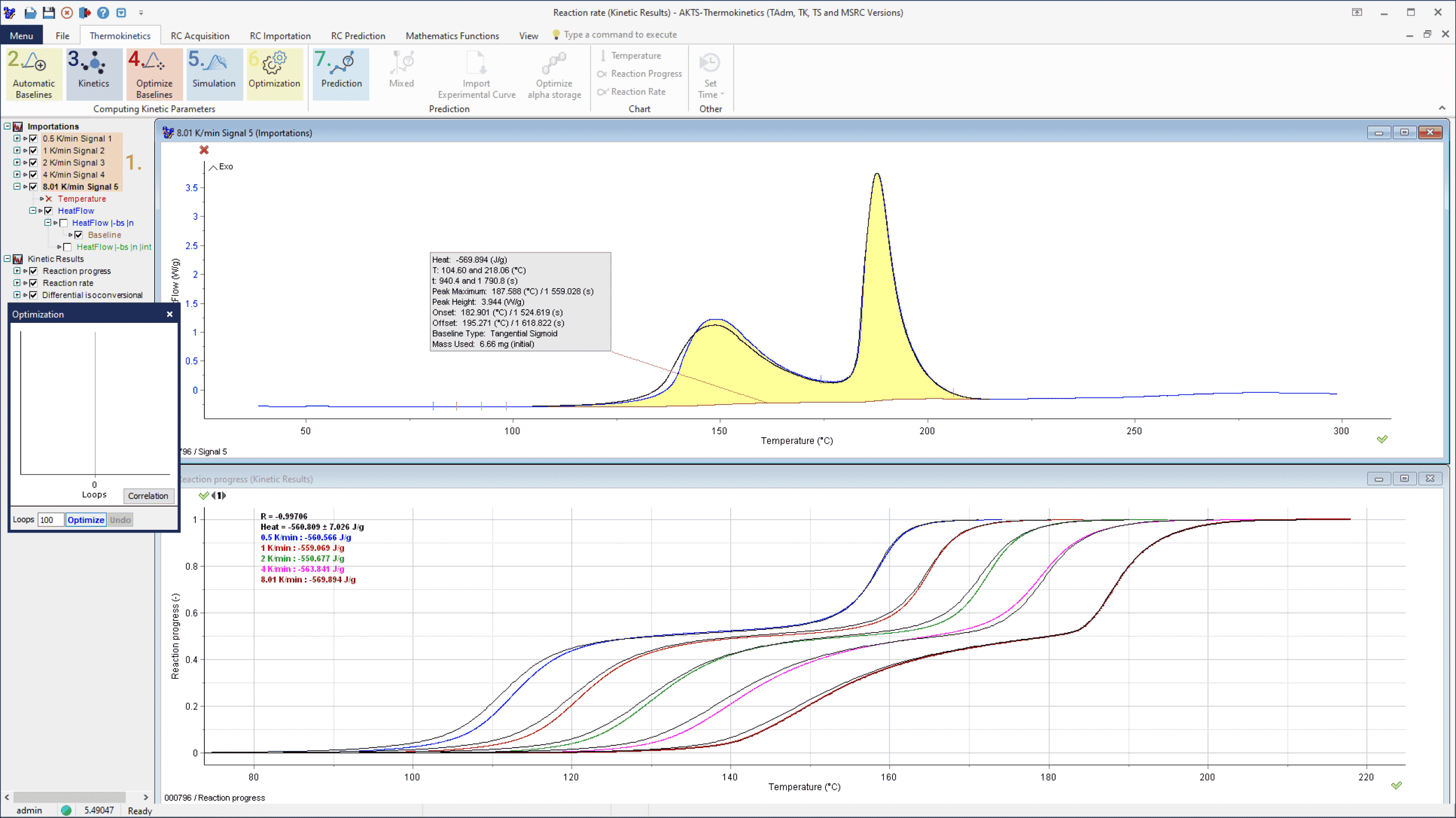
B(t) can be calculated iteratively. The convergence is achieved as soon as the relative average deviations between two iterations are smaller than an arbitrarily chosen value (for example 1E-6). A tangential area-proportional baseline calculated using arbitrarily 300 iteration loops is presented in Fig. 3, top section, was used for the evaluation of the dependence of reaction rate (middle) and reaction extent (bottom section) on the temperature.
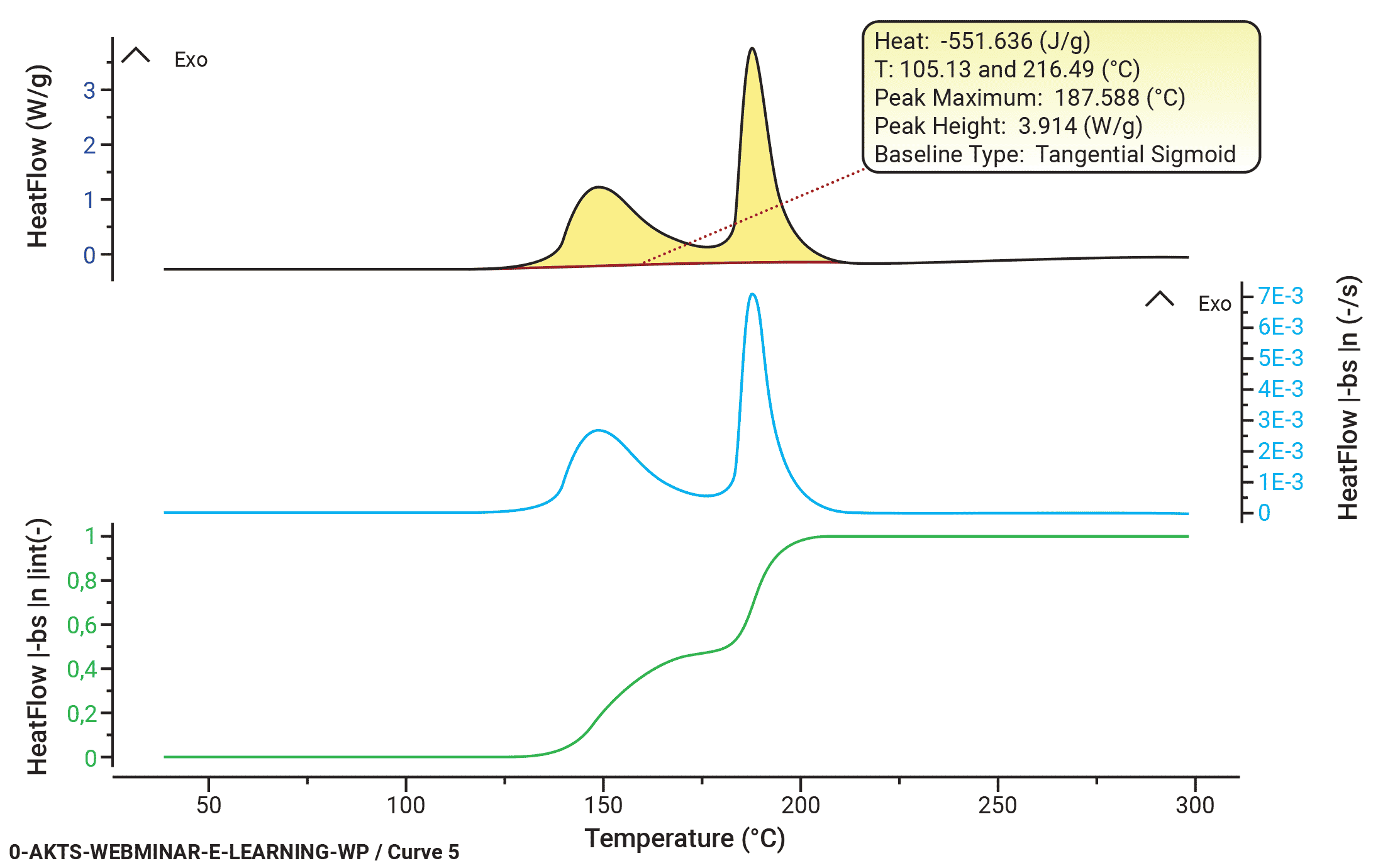
Fig. 3 – Evaluation of DSC signal collected at a heating rate of 8 K/min: (top) baseline construction, (middle) evaluation of the temperature dependence of the reaction rate and (bottom) reaction progress.
AKTS-Thermokinetics Software enables advanced baseline construction of 10 different baseline types (tangential sigmoid, tangential first point, tangential last point, sigmoid, spline, linear, horizontal first point, horizontal last point, equal to zero baseline, staged) because the correct baseline identification is one of the most critical parts of data treatment. Constructed baselines can be optimized numerically.
It is obvious that the baseline construction can significantly influence the computation of the kinetic parameters of the reaction. The detailed discussion of the influence of the baseline construction on the shape of the peak and value of the kinetic parameters is presented in the studies of Svoboda al. [10-13]. In certain cases (isoconversional approach) the error in determination of the activation energy can be in the range of 15-20% [11]. Advanced mathematical procedures are therefore necessary for the most appropriate baseline construction for each DSC signal.
Determination of the Kinetic Parameters (STEP 2)
Kinetic analysis of thermally stimulated processes
Chemical reaction rates are generally considered to be a function of two time-dependent variables, temperature T and reaction extent α (which varies from 0 to 1 from the beginning to completion of the reaction). The dependence of the reaction rate on the temperature is represented by the rate constant k(T) (at a given temperature) and on the reaction extent by the reaction model f(α) and is generally expressed as:
![]()
This equation relates the reaction rate dα/dt to three so-called kinetic parameters: the pre-exponential factor A, the activation energy E, and the reaction model f(α). Commonly, these three parameters are named as the kinetic triplet. Determination of the kinetic triplet is a prerequisite to establish a mutual relationship between the reaction rate dα/dt, the extent of conversion α, and the temperature (or time). The extent of the conversion α is determined experimentally as a fraction of the overall change in a physical quantity that represents the reaction progress as a function of time t or temperature T. If the reaction process is evaluated by monitoring of the heat flow, (DSC, calorimetry), then the extent of conversion at certain temperature or time is expressed as the ratio of the amount of evolved (or consumed) heat to the total amount of heat released (or absorbed) during the reaction. Similarly the reaction extent is evaluated from the experiments in which the change of the mass loss (TG) or any other quantity (e.g. the evolution of the gaseous species detected by MS or FTIR) are monitored during the reaction course. For adiabatic conditions the conversion can be expressed as the ratio of the observed temperature rise to the final adiabatic temperature rise.
The list of the commonly applied reaction models f(α) in the solid-state kinetics is presented in Table 1.
| Reaction model | Abbreviation: f(α) | Reaction model | Abbreviation: f(α) |
|---|---|---|---|
| first order | F1 : 1-α | Avrami-Erofeev | A1.5 : 1.5 (1-α) [-ln(1-α)]^(1/3) |
| second order | F2 : (1-α)^2 | Avrami-Erofeev | A2 : 2 (1-α) [-ln(1-α)]^(1/2) |
| third order | F3 : (1-α)^3 | Avrami-Erofeev | An : n (1-α) [-ln(1-α)]^(1-1/n) |
| nth order | Fn : (1-α)^n | contracting cylinder | R2 : 2 (1-α)^(1/2) |
| power law | P1 : α^0 | contracting sphere | R3 : 3 (1-α)^(2/3) |
| power law | P2 : 2 α^(1/2) | Rn : n (1-α)^(1-1/n) | |
| power law | P3 : 3 α^(2/3) | 1-dimensional diffusion | D1 : 1/(2α) |
| power law | P4 : 4 α^(3/4) | 2-dimensional diffusion | D2 : [-ln(1-α)]^-1 |
| power law | Pn : n α^(1-1/n) | 3-dimensional diffusion | D3 : 1.5 [1-(1-α)^(1/3)]^-1 (1-α)^(2/3) |
| autocatalytic | (1-α)^n α^m |
Table 1 – Generally applied reaction models f(α) in the solid-state kinetics
All types of the reaction models f(α) can be reduced to three major cases when considering the dependence of the reaction progress on the time in isothermal conditions: accelerating, decelerating and S-shaped, (sigmoidal, logistic, autocatalytic). Each of these types has a characteristic ‘reaction profile’ or ‘kinetic curve’, the terms frequently used to describe a dependence of α or dα/dt on t or T. Such profiles are readily recognized for isothermal data : the respective dependences of α or dα/dt vs. t for these three main cases in isothermal conditions are shown in Figure 4.
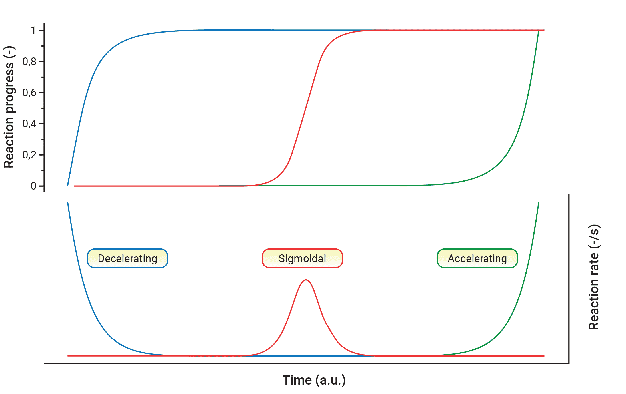
Fig. 4 – Relationship of the reaction progress α vs time in isothermal conditions for decelerating, sigmoidal and accelerating reaction models.
(1) Decelerating models represent processes in which the reaction rate in isothermal conditions has maximum at the beginning of the reaction and decreases continuously during the reaction course. The most common example of such behavior is presented in a reaction-order model:
![]()
where n is the reaction order. Diffusion models (Table 1) belong also to the decelerating models.
(2) Sigmoidal reaction models are characteristic for the reactions in which the accelerating and decelerating behavior occur at the beginning and at the end of the process, respectively. The maximum of the reaction rate is reached in some intermediate reaction extend.Typical sigmoidal kinetics describes the Avrami-Erofeev (A-E) or extended Prout-Tompkins (P-T) autocatalytic models (known also as truncated Sestak-Berggren model) having the following form:
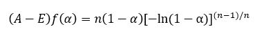
![]()
These reactions typically have a long induction period, in which the significant conversion α prior to detection of a signal may occur. Our studies demonstrate that conversion extent even smaller than 1% may significantly change the thermal behavior of a substance [14] therefore the thermal history of the sample must be considered during kinetic analysis. For sigmoidal reaction models in addition to the usual kinetic triplet, it is necessary to introduce the initial conversion α0 as an essential parameter required for the simulation of the thermal behavior of the materials. More information concerning this issue and explanation of the invented by AKTS Double-Scan Test (DST) will be presented in further part of the description of this AKTS Thermokinetics Software.
(3) Accelerating models represent processes whose rate increases continuously with increasing the extent of conversion α and reaches its maximum at the end of the process. Models of this type can be exemplified by a power-law model:
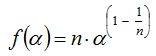
where n is a constant
The most general model that allow considering all three types of the conversion dependencies is known as Sestak and Berggren (SB) an empirical equation
![]()
in which the values of the exponents m, n, and p characterize the contribution of the different reaction models in the observed reaction rate. The SB model is generally used in truncated form (p=0) being equivalent to the so called Prout-Tompkins autocatalytic model.
One of the most important motivation for kinetic evaluation of the experimental data is the prediction of process rate and reaction progress at arbitrarily chosen values of temperature T or time t under any thermal mode (isothermal, non-isothermal, adiabatic, etc.). At laboratory scale the most common non-isothermal mode is one with an imposed heating rate dT/dt = β = constant, while for long-term storage diurnal and seasonal temperature variations might be experienced. Predictions in either case are reliable only when the sound kinetic analysis methods are used. It is however very important to note that a common difficulty in the correct interpretation of experimental data is that even an apparently simple one-step process may in reality contain multiple steps and may require more complex elaboration of the experimental results. This remark is illustrated in Figure 5 where unknown amount of sub-stages can contribute to the observed, apparently simple, shape of the heat flow signal.
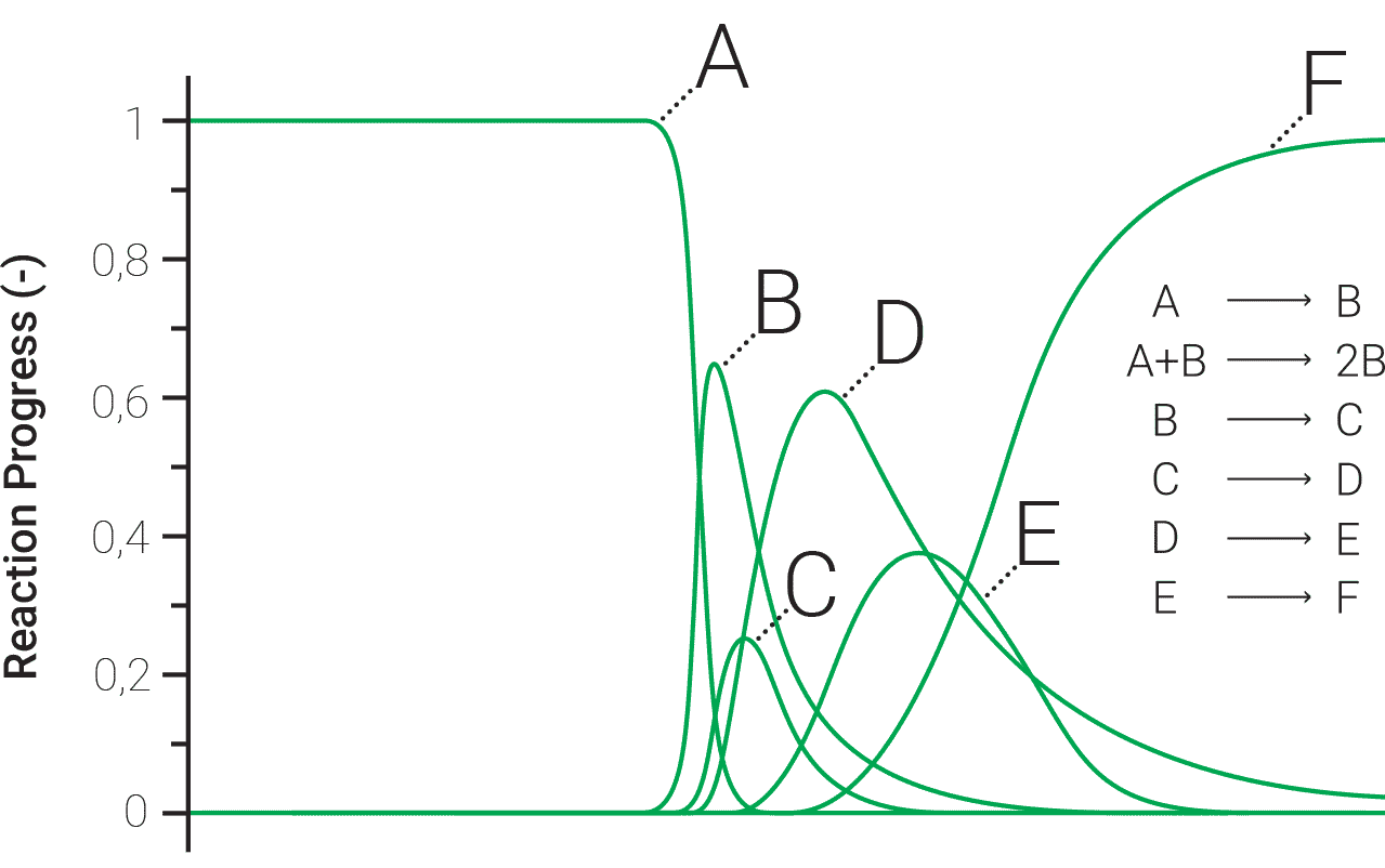
Observed thermal event can be the sum of thermal events created during certain stages of the reaction wich are not always know.
How many reactions may contribute to the observed DSC signal? 2? 4? 8?
Fig. 5 – The number of stages and physico-chemical reaction pathways contributing to the observed summary, i.e. experimentally recorded heat flow signal are generally unknown.
With the approach proposed in AKTS software it is possible to analyze observed thermal events that can be the combination of not always known chemical sub-stages of the reaction. For simplest reactions like A->B or for the reactions containing several consequent steps like:
A->B->C->D->E
AKTS Software uses an advanced differential isoconversional technique for evaluating kinetic parameters and use them for predictions. The differential isoconversional approach allows determination of kinetic parameters for all sub-reactions as a function of the conversion. This unique feature enables to describe very precisely processes combining parallel or consecutive steps because at each reaction extent the several elementary (usually unknown) processes may take place simultaneously. Therefore, AKTS Software avoids cumbersome, time consuming and sometimes very arbitrary approach introducing the assumption of existence of several reaction models and activation energy values necessary for the kinetic analysis of the investigated process. In certain cases, the isoconversional approach may describe the reaction course not precisely enough and better fit of experimental data can be obtained by model-fitting method. AKTS TK Software allows application also of this second kinetic approach.
More generally, the differential isoconversional method does not require an explicit assumption of the form of f(α), and additionally does not assume the constancy of A and E during the course of the process (see Fig. 3.3). It is therefore generally more precise than presupposing knowledge of f(α) and assuming that A and E are constant over the range of α from 0 to 1.
Since differential isoconversional methods do not make use of any approximations about reaction models they are potentially very accurate and avoid the risk of wrong model assumptions which are not correct from chemical point of view and can have very dangerous consequences for e.g. thermal aging or hazards evaluation. Another advantage is that with the differential isoconversional approach it is possible to correctly describe kinetics of complex reactions within few minutes only.
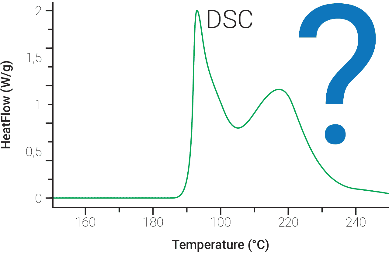
The isoconversional principle states that the reaction rate at a constant conversion α (i.e., the isoconversional rate) is only a function of the temperature. This can be easily demonstrated by taking the logarithmic derivative of the reaction rate at α = constant:
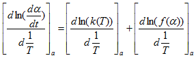
where the subscript α indicates isoconversional values, i.e., the values related to a given extent of the conversion α. Because at α =const, f(α) is also constant therefore the second term in the right hand side of the previous equation is zero. Thus:
It follows that the temperature dependence of the isoconversional rate can be used to evaluate isoconversional values of the activation energy, E(α) without assuming or determining any particular form of the reaction model f(α). For this reason, isoconversional methods are frequently called ‘model-free’ methods. However, one should not take this term literally. Although the methods do not need to identify the reaction model, they do assume that the conversion dependence of the rate obeys some f(α) model. This is visible with the most common differential isoconversional method of Friedman. Friedman proposed to apply the logarithm of the conversion rate dα/dt as a function of the reciprocal temperature at any conversion α:
![]()
![]()
f(α) is a constant in the last term at any fixed value of α and the dependence of the logarithm of the conversion rate dα/dt on 1/T shows a straight line with the slope m = -E/R and intercept equal to ln(A(α)·f(α)) as presented in Figures 6 to 8 by extension
![]()
with A'(α) = A(α)f(α)
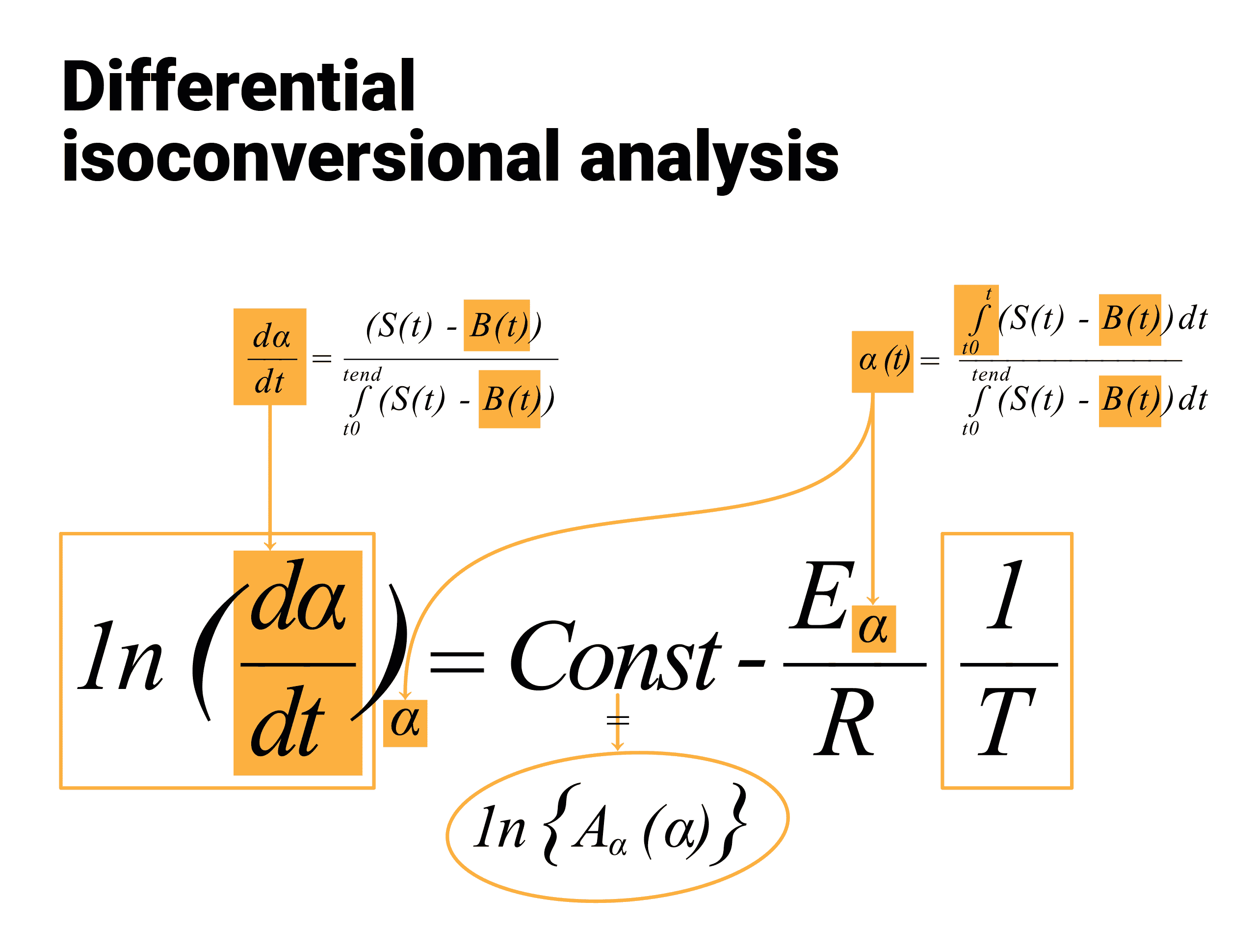
Fig. 6 – Differential isoconversional analysis: dependence of the reaction rate on the kinetic parameters at any reaction extent α.
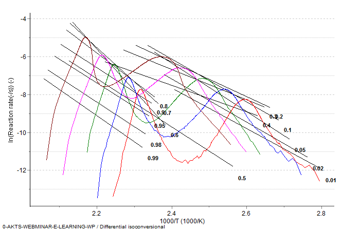
Fig. 7 – Differential isoconversional analysis: dependence of the reaction rate on temperature and the heating rate for the isoconversional points at which the reaction extents (marked by numbers between 0.01 and 0.99) are the same.
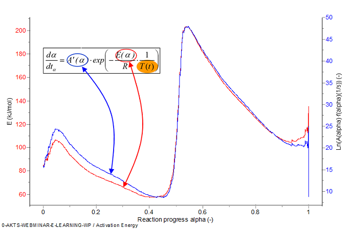
Fig. 8 – Activation energy and pre-exponential factor as a function of the reaction progress.
The dependence of the E and A on the reaction extent evaluated by the differential isoconversional analysis can be applied for accurate simulation of the reaction rate dα/dt and reaction progress α as illustrated in Figure 3.6. It is also possible to evaluate the time tα which is required to reach a given reaction progress α using the expressions:
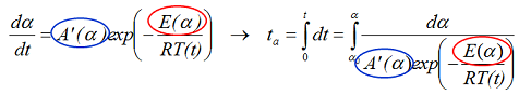
By extension above equation can be applied to calculate the reaction rate dα/dt and progress α for milligram, kilo, and ton scales under any thermal conditions, after introducing into the dependence T(t) the appropriate heat balance equations.
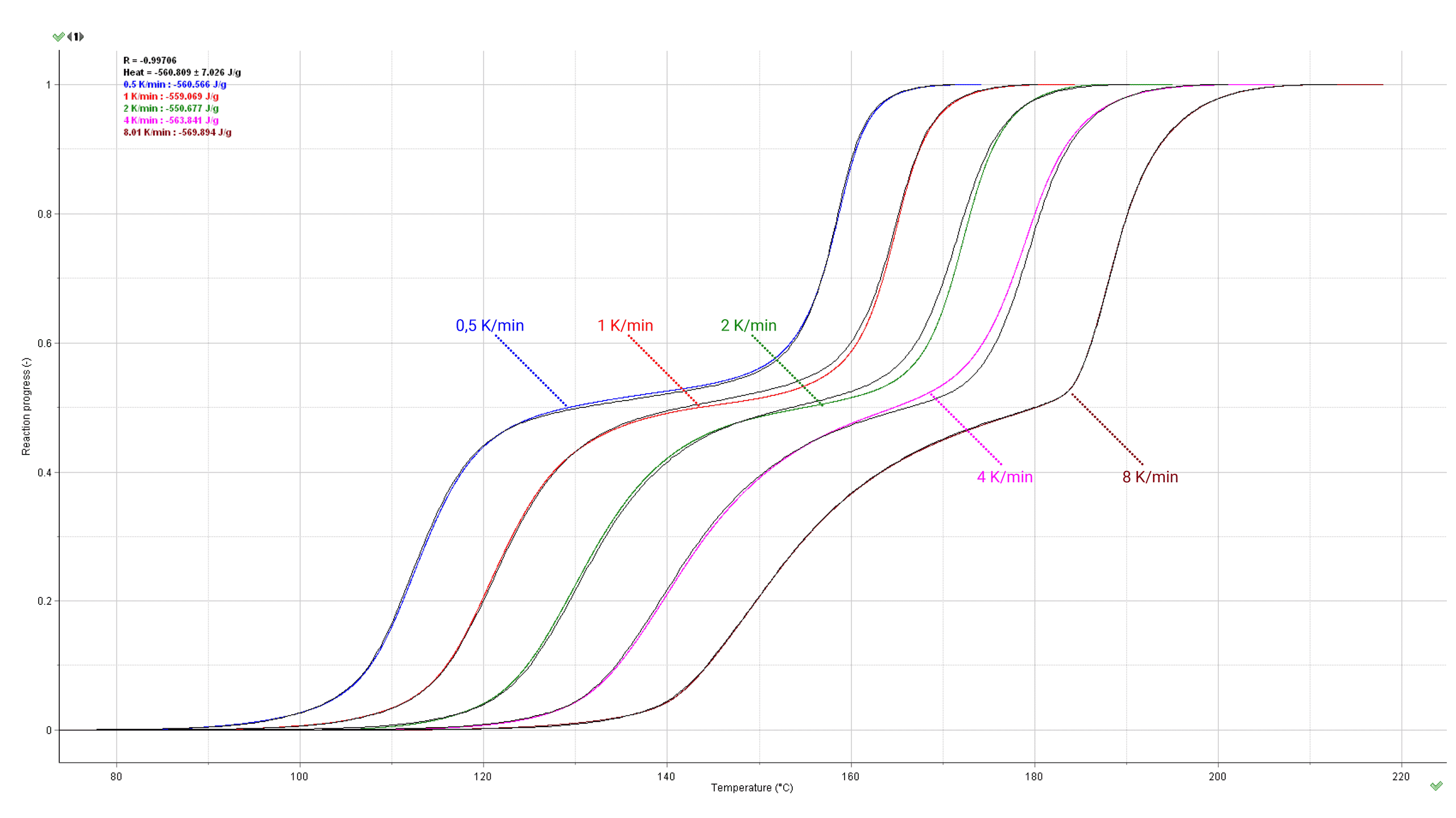
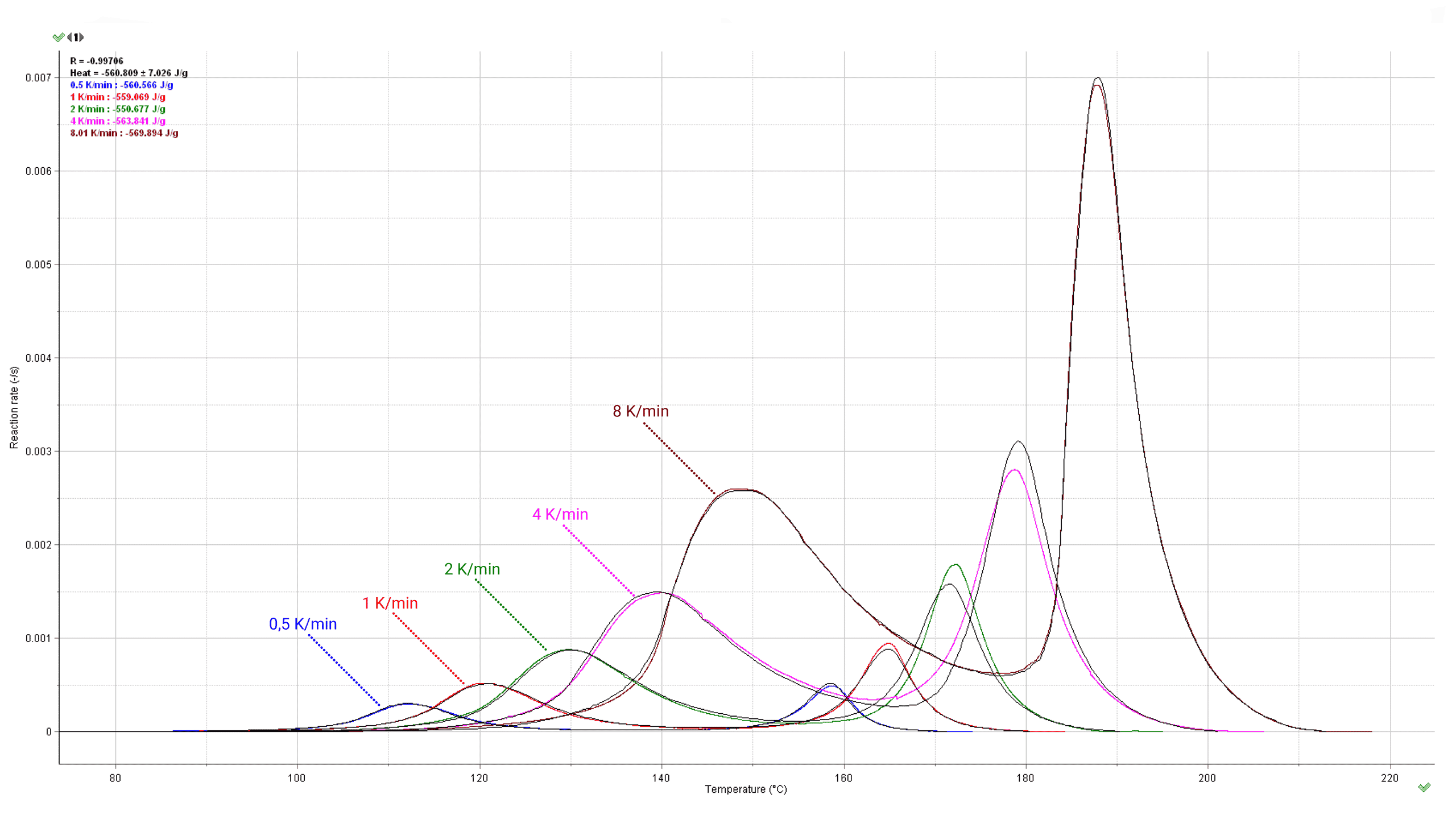
Fig. 9 – Comparison of experimental (color) and simulated (black lines) reaction rates (bottom) and progresses (top) for different heating rates (marked in K/min on the curves).
Basic information about isoconversional methods
A detailed analysis of the application of the various isoconversional methods (i.e. differential and integral) for the determination of the activation energy has been reported in the literature by Budrugeac [15]. The convergence of the activation energy values obtained by means of a differential method like Friedman method [16] with those evaluated by integral methods with integration over small ranges of reaction progress a comes from the fundamentals of the differential and integral calculus. In other words, it can be mathematically demonstrated that the use of isoconversional integral methods (for example: Ozawa-Flynn-Wall [17-18] can yield the systematic errors when determining the activation energies. These errors depend on the size of the ranges of reaction progress Δα over which the integration is performed. These errors can be minimized by using infinitesimal ranges of reaction progress Δα. As a result, isoconversional integral methods come closer to the differential isoconversional methods formerly proposed by Friedman [16].
The differential methods are based on the following reaction rate equation:
![]()
where β is the heating rate, T the temperature, E(α) the activation energy, A(α) the preexponential factor and f(α) is the differential form of the reaction model function.
As far as isoconversional integral methods are considered, these techniques are based on the equation:
![]()
where g(α) is the integral form of the reaction model function.
The isoconversional integral methods with the integration over low ranges of the degree of conversion and respectively temperature, are based on the equation:
which is derived by supposing that in the range of the variation of the reaction extent Δα, the activation energy E can be assumed constant. Obviously, the use of such an approach leads to a plot of E versus the reaction extent α. However, the activation energy as a function of the conversion progress looks like a stair function in which the low ranges of Δα where E keeps a constant value are clearly marked. The number of stairs depends directly on the size of Δα.
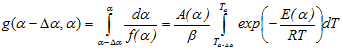
In order to evaluate the integrals from the previous equation, one can use the theorem of the average value, we obtain:
where
![]()
and
![]()
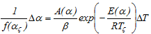
Since the number of stairs (where the activation energy E is assumed to be constant) depends directly on the range of chosen Δα, then an unlimited number of stairs can be reached by making Δα infinitesimal. For Δα → 0, we have Tξ → T and f(αξ) → f(α). As a consequence, the previous equation turns back into its differential form:
![]()
It means that the isoconversional integral methods come close to isoconversional differential method which corresponds to the Friedman approach that is described in the previous chapter. The conversion rate expression can now be adapted to an arbitrary variation of temperature by replacing β(dα/dT) with dα/dt.
| Nomenclature | |
|---|---|
| A | pre-exponential factor |
| A’ | modified pre-exponential factor A'(α)=A(α)·f(α) |
| E | activation energy |
| k(T) | rate constant |
| R | ideal gas constant |
| t | time |
| T | Temperature |
| α | reaction progress |
| α0 | initial reaction progress at t=0 |
| β | imposed heating rate dT/dt |
| DSC | Differential Scanning Calorimeter |
Application of kinetic parameters for the simulation of the reaction course, evaluation of the thermal aging and shelf life (STEP 3)
Prediction of the reaction progress under any temperature mode
The DSC data collected during non-isothermal experiments carried out with different heating rates were used for determination of the kinetic parameters and thereafter applied for prediction of the reaction extent for any temperature mode such as:
- Isothermal, non-isothermal, stepwise
- Modulated temperature or periodic temperature variations
- Rapid temperature increase (temperature shock)
- Real atmospheric yearly temperature profiles with daily minimal and maximal fluctuations. TK Software allows predictions for 50 climates available in the default version.
- NATO norm STANAG 2895 temperature profiles: Zones A1, A2, A3, B1, B2, B3, C0, C1, C2, C3, C4, M1, M2, M3.
- Customized temperature profiles
- Sample Controlled Thermal Analysis (SCTA)
Isothermal, non-isothermal, modulated, stepwise and real atmospheric temperature modes
Isothermal
Kinetic parameters calculated from non-isothermal experiments allow prediction of the reaction progress at any temperature mode: isothermal, non-isothermal and intermediate intervals in the heating rate, expressed, e.g. in oscillatory temperature modes. The prediction of the reaction progress and rate in isothermal temperature mode in the range of 50-95°C is depicted below:
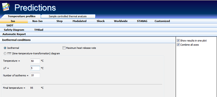
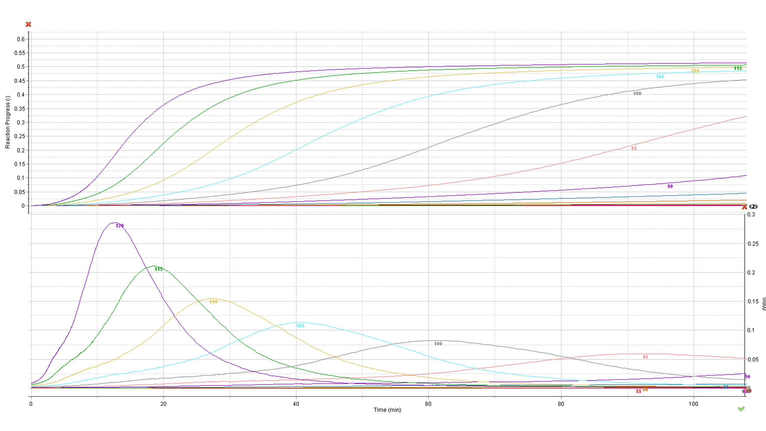
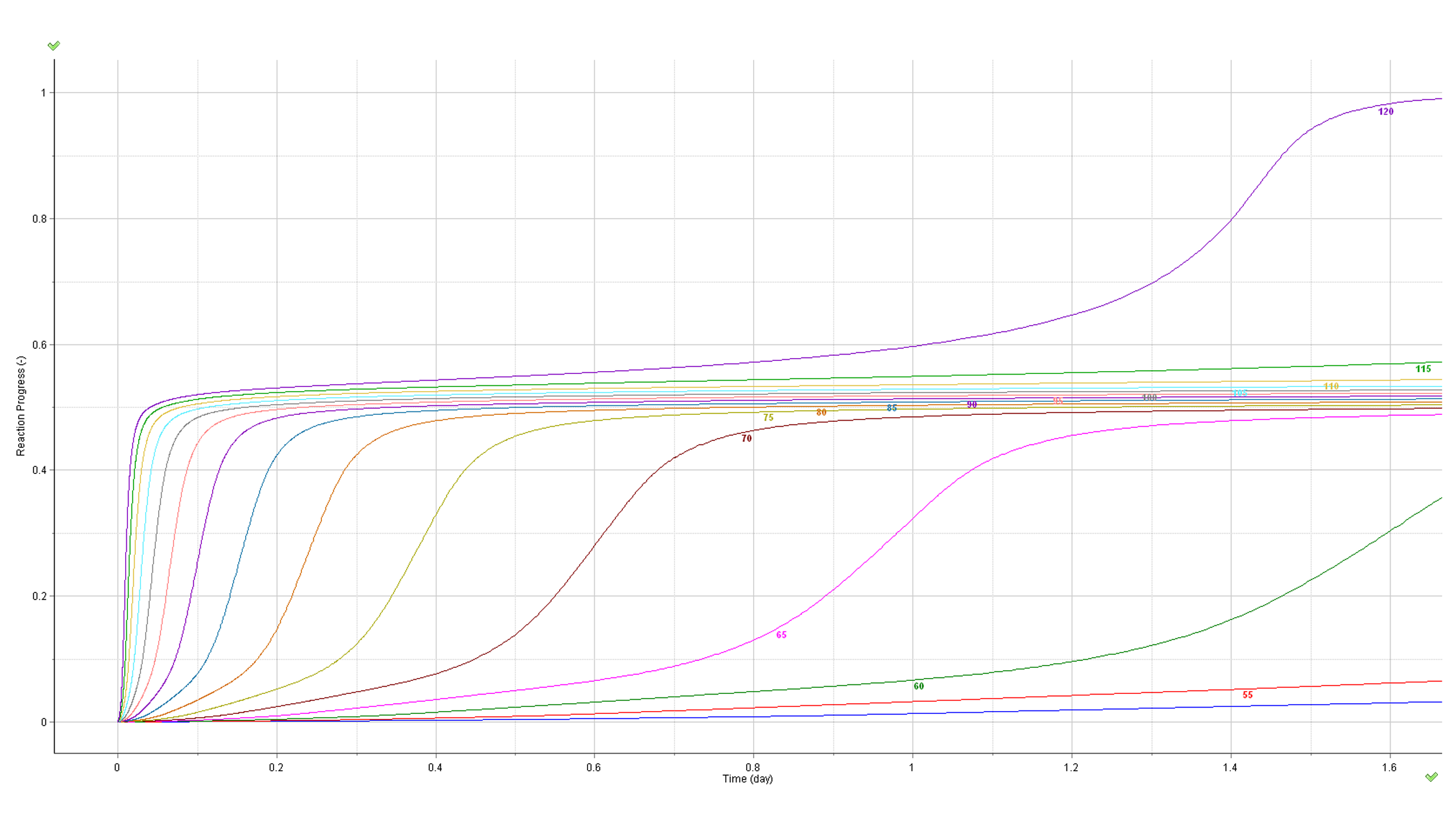
Fig. 10 – Calculated reaction rate and progress (normalized signals) as a function of time under isothermal conditions. The values of the temperature in °C are marked on the curves.
Non-Isothermal
In general, non-isothermal scans with different heating rates are carried out within a much wider temperature range than it is possible, from the experimental reasons, in isothermal conditions. This allows to discern between the different reaction paths involved in the kinetic description of the process. Non-isothermal data contain the necessary information on the time-temperature dependence of particular processes which is a prerequisite for the correct identification of the complex nature of the investigated reaction. Computations are usually made with the results obtained from at least 4-5 heating rates such as 8, 4, 2, 1, 0.5 K/min with a ratio of 8/0.5= 16 between the highest and lowest heating rates. The application of heating rates too close to each other should be avoided. If they are too close, they become tantamount to an unacceptable model-fitting analysis using single heating-rate data (see ICTAC kinetic projects [2-7]). Our general tip for experimental data is following: one should start the kinetic experiments with the heating rate of e.g. 4-5 K/min. It enables to quickly examine the shape of the signal over the whole temperature range. Then continue by 8 K/min and 2 K/min. If signal to noise ratio is not good for 2 K/min the sample mass should be increased, following experiments should be carried out with heating rates of 1 K/min and 0.5 K/min.
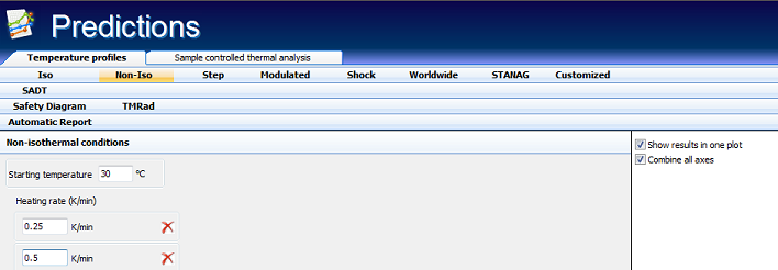
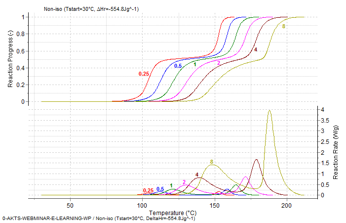
Fig. 11 – Calculated reaction rate and progress (normalized signals) as a function of temperature under non-isothermal conditions. The values of the heating rates in K/min are marked on the curves.
Stepwise
This temperature mode combines the features of iso- and non-isothermal experiments. The user has possibility to predict the reaction course (reaction rate and reaction progress) occurring during the sequence of iso- and non-isothermal temperature periods. The durability of the certain reaction zones, the temperatures and heating (cooling) rates applied are fully customizable
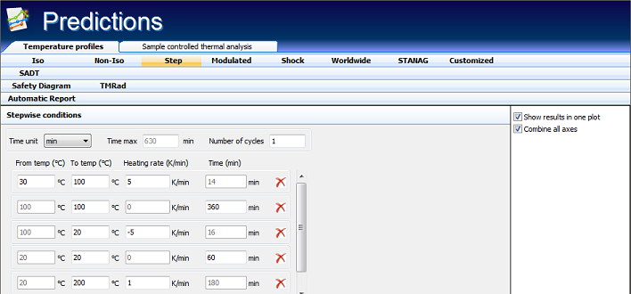
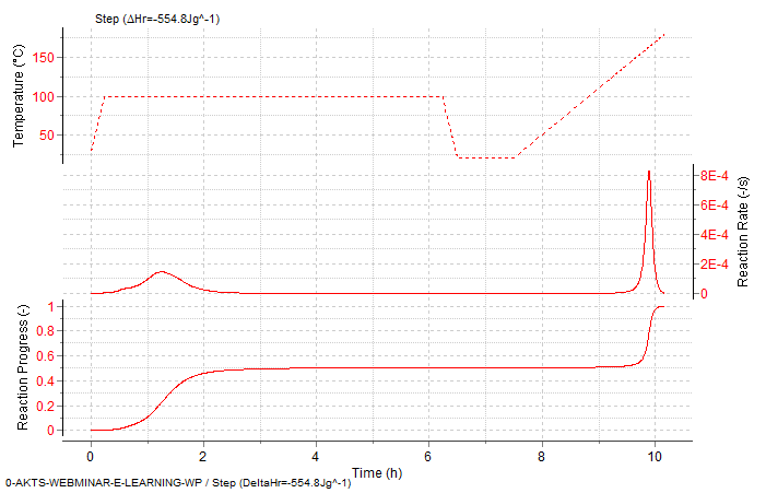
Fig. 12 – Stepwise mode. Reaction rate and progress α (normalized signals) as a function of time for subsequent isothermal and non-isothermal temperature zones.
Modulated
Examples of predictions of the reaction progress in an oscillatory temperature mode (widely applied in temperature-modulated calorimetry) are given below. A temperature-modulated mode increases the basic understanding of the characterization of materials.
Even if, the arithmetic mean temperature (30°C) is the same in both experiments (red-isothermal, blue the oscillatory temperature mode) one observes the distinct differences of the reaction courses. The presence of temperature amplitudes greatly increases the reaction progress and rate. The prediction of the reaction course at 30°C and at 30°C with ± 20°C amplitude and period of 24 h is presented below
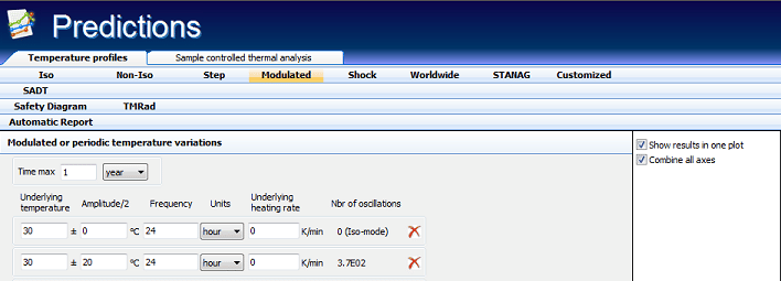
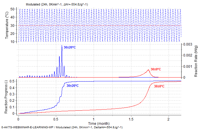
Fig. 13 – Reaction rate (middle) and reaction progress (bottom, normalized signals) as a function of time under isothermal (red curves, 30°C) and oscillatory (blue curves, 30°C±20°C, period 24 h) temperature conditions.
Real atmospheric temperature mode
Prediction of the reaction rate and progress for real atmospheric temperature profiles allows the investigation of the properties of low-temperature decomposed substances under different climates (yearly temperature profiles with daily minimal and maximal fluctuations). The important goal of the investigation of thermal decomposition kinetics is the need to determine the thermal stability of substances, i.e. the temperature range over which a substance does not decompose with an appreciable rate. The correct prediction of the reaction progress of materials which are unstable under ambient conditions (food, drugs, some polymers, etc.) requires accurate application in the calculations of both:
- The kinetic parameters
- The exact temperature profile for a given climate
Calculations can be achieved for any fluctuation of the temperature which makes possible the predictions of thermal stability properties for varying climates. Exact consideration in the calculations of daily minimal and maximal temperature variations of worldwide climates provides very valuable insight when interpreting and quantifying the reaction progress of materials subjected to atmospheric conditions.
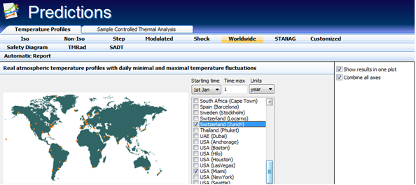
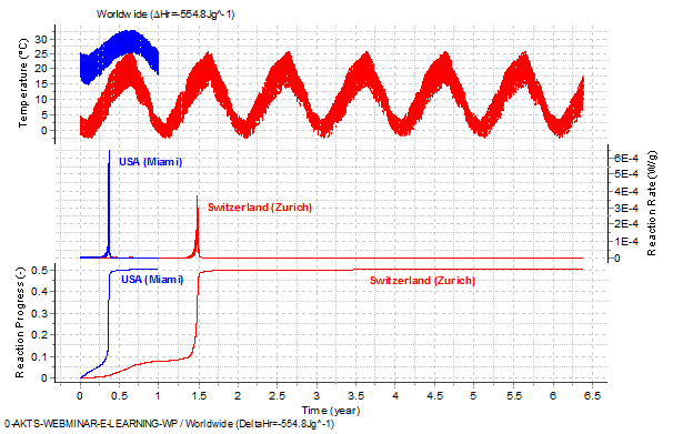
Fig. 14 – Top: Average daily minimal and maximal temperatures recorded between 1961 and 1990 in Zurich (red) and Miami, USA, (blue ). Middle and bottom: Reaction rate and reaction progress (normalized signals) as a function of time for the Zurich and Miami temperature profiles.
STANAG 2895
The application of kinetics makes possible the precise prediction of the reaction progress under temperature mode corresponding to real atmospheric changes according to STANAG 2895 [19]. During their production, storage or final usage, chemicals often undergo temperature fluctuations. Due to the fact that the reaction rate varies exponentially with the temperature it is important that predictive tools could enable the simulation of the reaction progress in the real conditions, as a small temperature jump can induce a significant increasing reaction rate.
The STANAG 2895 describes the principal climatic factors which constitute the distinctive climatic environments found throughout the world and provides guidance on the drafting of the climatic environmental clauses of requirement documents. The knowledge of temperature profiles described in STANAG 2895 helps in the prediction of the influence of the temperatures on the slow rate of decomposition of e.g. high energetic materials such as propellants. The precise prediction of the reaction rate and progress requires the knowledge of the diurnal and annual variations of the meteorological and storage /transit temperatures. The meteorological temperature represents the ambient temperature measured under standard conditions, whereas storage and transit temperature represents the air temperature measured inside temporary unventilated field shelter e.g. in railway boxcar which is exposed to direct solar radiation. Applying the advanced kinetic software it is possible to calculate the reaction progress using the kinetic parameters determined from thermoanalytical signal and taking into account the dependence of the temperature changes depicted in STANAG 2895.
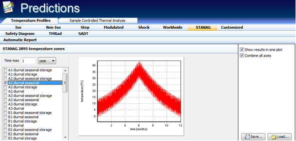
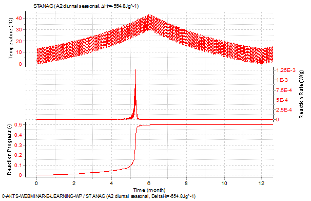
Fig. 15 – Predictions of the reaction rate (middle) and reaction progress (bottom) as a function of time during the temperature variations (top) represented by the diurnal storage temperature profiles of climatic category A2 of STANAG 2895.
Customized Temperature Profiles
The TK Software allows the precise simulation of the reaction course at any temperature profile, even those close to the ambient temperatures. The simulation of the reaction progress for temperature profile corresponding to the temperature fluctuations measured during the sample storage is presented in the figure 16. Such predictions are of great importance for evaluation of the shelf life of the materials which may slowly decompose even at ambient temperatures.
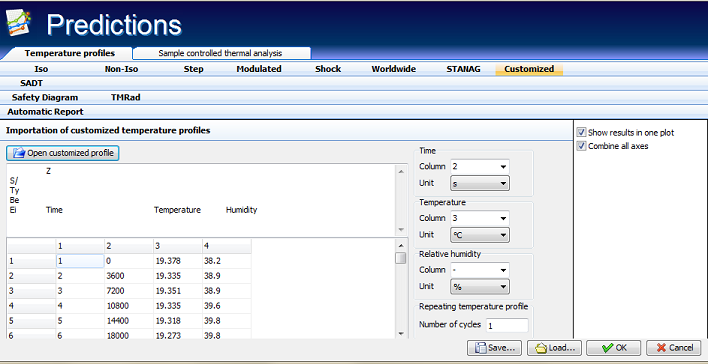
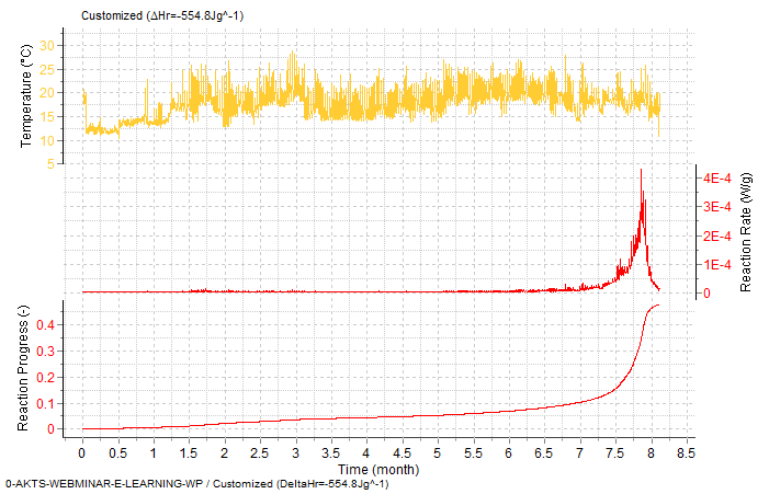
Fig. 16 – Prediction of the reaction rate (middle-) and reaction progress (bottom curve) during severe variations of the temperature profile (top). The simulation of the reaction course can be performed for any, user introduced time-temperature data.
Sample Controlled Thermal Analysis (SCTA)
AKTS-Thermokinetics Software can optimize temperature program in such a way that it allows to assure the value of the reaction rate set by the user. It is often the case in industrial applications, that in order to achieve a certain, specific sample properties, the reaction rate should be very carefully controlled, not exceeding e.g. a certain critical value. This method of controlling reaction rate is known as Sample Controlled Thermal Analysis.
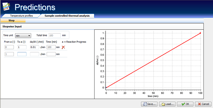
Therefore, as powerful tool for the solution of such problems, AKTS-Thermokinetics Software contains tools which through kinetic analysis allow to permit the rate controlled mass change for thermogravimetric signals, rate controlled conversion and/or rate controlled partial area for DSC measurements. The purpose of TK Software in SCTA mode is to provide such temperature profiles which result in constant mass loss rates in TGA experiments or rate controlled heat release (or consumption) in DSC measurements.
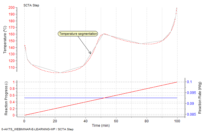
Fig. 17 – Prediction of rate controlled conversion in Sample Controlled Thermal Analysis mode: the dependences temperature vs time (top), reaction rate and reaction extent vs time (middle) and reaction extent vs temperature (bottom).
References
[1] AKTS AG, https://www.akts.com AKTS-Thermokinetics Software. The Swiss Institute for the Promotion of Safety and Security (http://www.tuev-sued.ch/ch-en/activity/testing-equipment/dsc).
[2] M.E. Brown et al. Computational aspects of kinetic analysis. The ICTAC Kinetics project data, methods and results. Thermochim. Acta, 355 (2000) 125.
[3] M. Maciejewski, Computational aspects of kinetic analysis. The ICTAC Kinetics Project – The decomposition kinetics of calcium carbonate revisited, or some tips on survival in the kinetic minefield. Thermochim. Acta, 355 (2000) 145.
[4] A. Burnham, Computational aspects of kinetic analysis. The ICTAC Kinetics Project – multi-thermal-history model-fitting methods and their relation to isoconversional methods. Thermochim. Acta, 355 (2000) 165.
[5] B. Roduit, Computational aspects of kinetic analysis. The ICTAC Kinetics Project – numerical techniques and kinetics of solid state processes. Thermochim. Acta, 355 (2000) 171.
[6] S. Vyazovkin, A.K. Burnham, J.M. Criado, L.A. Pérez-Maqueda, C. Popescu, N. Sbirrazzuoli, ICTAC Kinetics Committee recommendations for performing kinetic computations on thermal analysis data, Thermochim. Acta, 520 (2011) 1-19.
[7] S. Vyazovkin, K. Chrissafis, M.L. Di Lorenzo, N. Koga, M. Pijolat, B. Roduit, N. Sbirrazzuoli, J.J. Suñol, ICTAC Kinetics Committee recommendations for collecting experimental thermal analysis data for kinetic computations, Thermochim. Acta, 590 (2014) 1-23.
[8] https://www.tuev-sued.ch/ch-de/leistungen/sicherheitspruefgeraete/dsc-cells , Accessed 09 June 10, 2020.
[9] W.F. Hemminger, S.M. Sarge, J. Therm. Anal., 37 (1991), 1455-77, The baseline construction and its influence on the measurement of heat with differential scanning calorimeter.
[10] R. Svoboda, J. Màlek, J.Therm.Anal. Calorim., 124 (2016) 1717-25, Importance of proper baseline identification for the subsequent kinetic analysis of derivative kinetic data, part 1.
[11] R. Svoboda, J.Therm.Anal. Calorim., 131 (2018) 1889-97, Importance of proper baseline identification for the subsequent kinetic analysis of derivative kinetic data, part 2.
[12] R. Svoboda, J.Therm.Anal. Calorim., 136 (2019) 1307-14, Importance of proper baseline identification for the subsequent kinetic analysis of derivative kinetic data, part 3.
[13] R. Svoboda, Thermochim. Acta, 655 (2017) 242-250, Linear baseline interpolation for single-process DSC data- yes or no?
[14] B. Roduit, M.Hartmann, P.Folly, A.Sarbach, Chem. Eng. Transactions, 31(2013) 907-912, Parameters Influencing the Correct Thermal Safety Evaluations of Autocatalytic Reactions.
[15] P. Budrugeac, J. Therm. Anal., 68 (2002) 131-139. Differential non-linear isoconversional procedure for evaluating the activation energy of non-isothermal reactions.
[16] H. L. Friedman, J. Polym. Sci, Part C, Polymer Symposium (6PC), 183-195 (1964), Kinetics of Thermal Degradation of Char-Forming Plastics from Thermogravimetry. Application to a Phenolic Plastic.
[17] T. Ozawa, Bull. Chem. Soc. Japan, 38 (1965) 1881-86. A new Method of analyzing Thermogravimetric data.
[18] J.H. Flynn, L.A. Wall, J. Res. Nat.Bur. Standards, 70A (1966) 487-523, General treatment of the thermogravimetry of polymers.
[19] STANAG 2895 (1990), Extreme climatic conditions and derived conditions for use in defining design/test criteria for NATO forces material, https://www.nato.int/cps/su/natohq/publications.htm.