Detailed description

SPECIFIC MIGRATION LIMITS Software (SML)
Employing advanced numerical algorithms, migration modelling with the SML software [1] allows prediction of the amount of organic migrant (like residual monomers, additives, contaminants, reaction products, non-intentionally added substances from plastic multi-layer or multi-material multi-layer materials) which migrate into the packed food or other contact media like pharmaceuticals, cosmetics, drinking water or environment. The application of the software insures the compliance of plastic food contact materials and articles with specific migration limits according to EU Regulations [2, 3] and Swiss Legislation [4].
The technique allows the specific migration assessment for complex materials, with different geometries and any multi-layer structure. Simulation of the migration process is based on Fick’s 2-nd law of diffusion under consideration of partitioning between adjacent layers or contact media in closed systems [1-4].
Temperature dependence of the diffusion process is considered by the Arrhenius equation. Diffusion coefficients of migrants in polymers are estimated by generally recognized estimation procedures (Piringer model) based on polymer specific constants (AP-values) [2] which are available for certain polymers. Extension of the AP value model by Brandsch for estimation of diffusion coefficients based on the glass transition temperature of polymers opens modelling opportunities for any polymer or polymer mixture by applying a glass transition temperature.
Estimation of partition coefficients between contact layer and contact medium (e.g. polymer and food simulant or water) is based on the migrants polarity expressed by the octanol/water partition coefficient of the migrants [5].
Time dependent migration curves and the concentration profile inside all layers of multi-layer structures can be computed for both, migrant from the material and from the contact medium.
The software allows the simulation of release of migrants from multi-layer materials in extended temperature ranges and/or under changing temperature conditions. Complex surrounding temperature profiles can be considered such as stepwise, modulated, temperature shock and additionally for temperature profiles reflecting real atmospheric temperature changes (yearly temperature profiles of different climates with daily minimal and maximal fluctuations).
Exposure and Compliance
Exposure
The consumers are likely to be exposed to a range of different products or articles containing migrants (chemicals) present in a large variety of packing materials. The safety concern of the total consumer exposure to migrants from all identified pathways form the basis for exposure assessment. The most important exposure pathways are food, household dust, indoor air and dermal contact with different polymer materials.

Fig. 1 – Total consumer exposure. The most important exposure pathways are food, indoor air, and dermal contact with different polymer materials.
Migrants with safety concerns are present in final products and articles at a level to accomplish the required technical effect. Due to interaction between materials and contacting media and thermodynamic driving forces these compounds are transferred by release (migration and emission) and/or distribution (partitioning) to food, the ambient air, or directly to the consumer through the dermal contact. The amount of compounds transferred is determined by the conditions of use (time and temperature, area to volume ratio) of the final products or articles. Typically exposure factors and/or thermodynamic parameters (partition and diffusion coefficients) are used to model the exposure scenarios. Due to the specific, individual habits and consumption behavior the consumer is exposed only to a limited extend to the individual pathways, therefore their specific contributions in terms of real exposure levels must be considered. Migrants with safety concerns are present in final products and articles at a level to accomplish the required technical effect. Due to interaction between materials and contacting media and thermodynamic driving forces these compounds are transferred by release (migration and emission) and/or distribution (partitioning) to food, the ambient air, or directly to the consumer through the dermal contact. The amount of compounds transferred is determined by the conditions of use (time and temperature, area to volume ratio) of the final products or articles. Typically exposure factors and/or thermodynamic parameters (partition and diffusion coefficients) are used to model the exposure scenarios. Due to the specific, individual habits and consumption behavior the consumer is exposed only to a limited extend to the individual pathways, therefore their specific contributions in terms of real exposure levels must be considered.
Interaction
Interaction between polymeric materials and contacting media results in a transfer of migrants (chemicals) from the materials to the media resulting in changes of their quality/properties with time and therefore is one of the key issue for quality assurance.
Depending on factors like the concentration, mobility and solubility in the polymeric material as well as the temperature and duration of the contact, the migrants inevitably migrate into the contacting medium what changes the medium composition with time. Migration of the migrants from complex materials and articles like multilayer packaging or composites are considered as a succession of individual mass transfer processes from which the slowest one defines the overall time scale. In most cases of practical relevance the diffusion process within the contact material is the rate determining step of the migration process. On the other hand the relationship between the solubility of a migrant in the material and the contacting medium, i.e. the partitioning process, strongly influences the overall amount of a migrant migrating into the medium and consequently the amount of migrant still left in the contact material.
Compliance
Realistic evaluation of the health risk associated with use of polymeric materials and articles is necessary. The risk-to-benefit ratio regarding the use of polymeric materials is negligible compared to the scenario of not using them. Even though this is unarguable, care must be taken to ensure consumer safety. Thus every regulation should consider the following points: i) the transfer of migrants from polymeric materials and articles to contacting media may be undesirable and ii) unavoidable mass transfer from state-of-the-art products should not be prohibited, if the migrants do not constitute health hazard and are technically required in an optimized system. The principal optimization criteria for modern products are their technical properties, consumer safety, environmental compatibility, and low cost. Fulfilling these criteria benefits the consumer and encourages technological progress.
Beside the acute toxicological properties of migrants, their chronic mutagenic and carcinogenic activity is the most important. The application to humans of the results of “No Observed Adverse Effect Level” (NOAEL) experiments on animals and the validity of subsequently derived “Acceptable Daily Intake” (ADI) values may be uncertain. “Estimated Daily Intake” EDI levels have additional uncertainties arising from regional and temporal considerations. The relevant exposure varies with season, geographic, and socioeconomic or ethnic background. The amount of migrants transferred from the polymeric materials and articles contacting media and hence the consumer exposure can vary over a large range. The theory of diffusion can be used to estimate mathematically the quantity of migrants transferred. However, many other complex factors affecting migration cannot be anticipated.
Compliance with worldwide regulations like FDA’s Code of Federal Regulation, EU Regulations and Directives, German BfR Recommendations, etc. is compulsory for polymeric materials and articles regarding positive listing and associated limits. The permissible levels of components to which the consumer is exposed are in focus of above considerations. All migrants can be divided into categories according to their health risk, which than can be used as a basis for regulation. On the one hand, the spectrum consists of migrants that pose no risk (those migrants which are inert or naturally occurring and are toxicological inactive) whereas on the other hand, there are migrants that must be excluded from use because they are recognized as toxicologically dangerous. Between this two extremes are placed the remaining migrants. They require toxicological or/and migration studies which will result in evaluation of the specific acceptable limits which should be taken into account during their use.
The verification of compliance of food contact materials by the application of recognized diffusion model was introduced 2002 in the European legislation [1].
References
[1] EU legislation Plastics Directive 2002/72/EC.
[2] EU legislation Plastics Directive N°10/2011
Migration modelling
Introduction
Polymeric materials (Plastics, Coatings, Rubbers, etc.) transfer their components (low molecular weight migrants like monomers, additives, etc.) to contacting media due to thermodynamic driving forces. This phenomenon is called mass transfer and its common wording is migration and/or emission depending on the type of contacting medium, i.e. liquid or gaseous. Due to transfer of migrants (chemicals) from the polymeric material to the contact medium their concentration in the polymeric material decreases and a new concentration profile is established. The amount of migrants is depleted first at the material/medium interface. The release of the migrants from polymeric materials to contacting media obeys in most cases the law of diffusion because the diffusion process is the rate determining step. In case of gaseous contact media the evaporation process may become under certain circumstances the rate determining step. It is obvious that mass transfer can occur as well from the contacting medium to the polymeric material.
The release of migrants from the polymeric material was generally assessed by experimental testing under conventional test conditions. Recently, due to better understanding of the mass transfer processes and application of advanced computational tools the simulation of the migration processes became the method of choice.
Simulation & diffusion models
The simulation of the complex migration process (mass transfer) is reduced to the evaluation of the rate determining step, i.e. the diffusion process. Correspondingly, migration modelling is based on application of the diffusion models. The migration process may be simulated according to real use conditions or according to conventional test conditions. Modelling migration according to conventional test conditions allows direct comparison between simulation and experimental results.
From mathematical point of view the system polymeric material – contact medium can be described by the 2-nd law of diffusion.
![]()
Fig. 2 – 2nd law of diffusion
To simplify the mathematical problem it is assumed that the polymeric material and its individual layers as well as the contacting medium are arranged parallel to each other. The diffusion equation being a partial differential equation can be solved with recognized numerical algorithms. With the numerical solution of the diffusion equation the migration kinetics, i.e. the rate of migration of migrants from the polymeric material to the contacting medium and the concentration profile of the migrants as a function of time can be calculated.
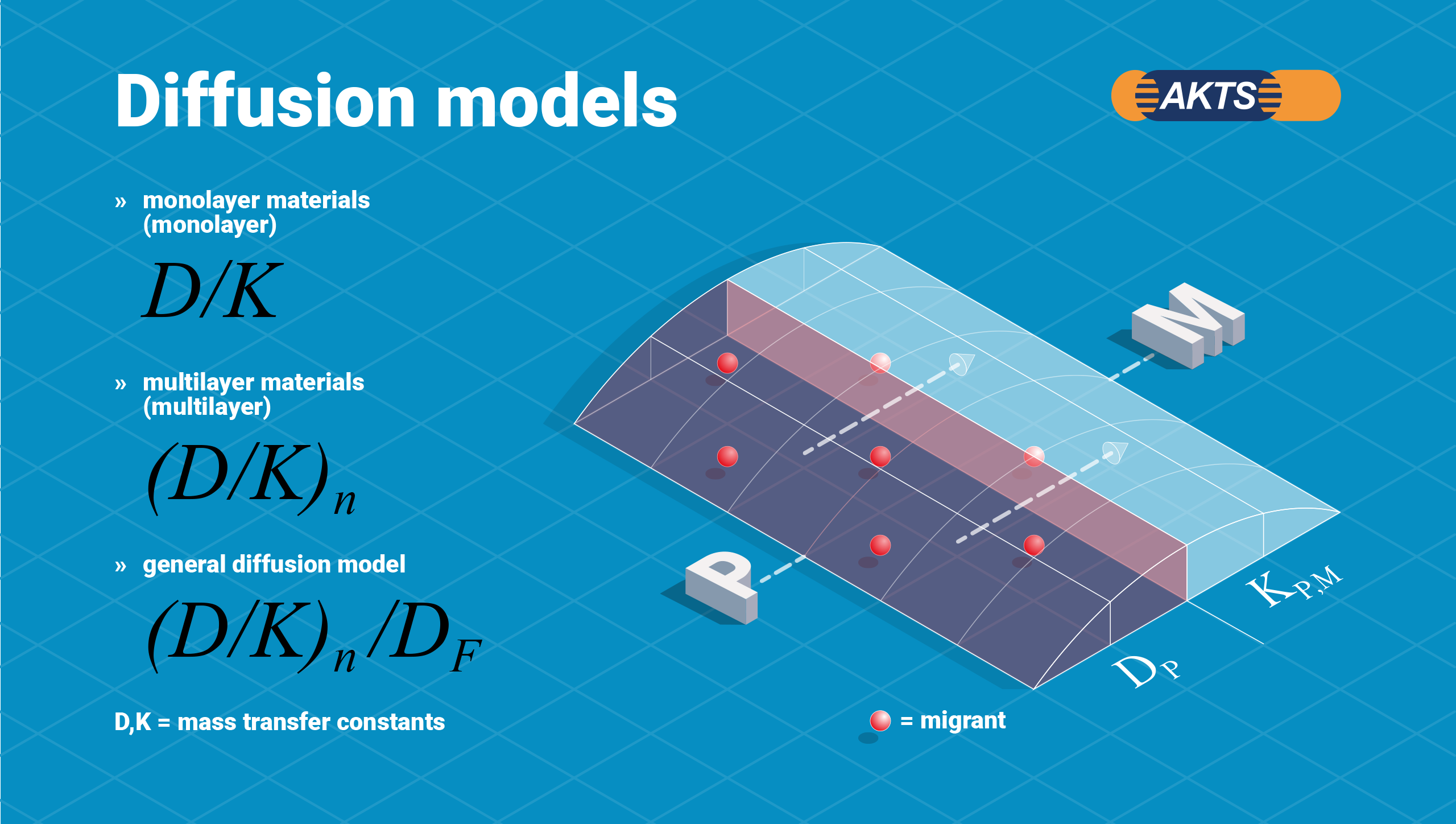
Fig. 3 – Diffusion models (n – number of layers, D – diffusion coefficient, K – partition coefficient)
One has to distinguish between monolayer and multilayer materials. If monolayer materials are in contact with a liquid medium, the system is described by two mass transfer constants, the diffusion coefficient (D) of the migrant in the polymeric material and the partition coefficient (K) of the migrant between polymeric material and contacting medium.
If multilayer materials with n layers are in contact with a liquid medium, all mass transfer constants describing the system must be considered, i.e. n diffusion coefficients of the migrants in each layer. As long as the contacting medium is a liquid or a gas the diffusion process in the medium is neglected because the diffusion rates are much higher compared to solids like polymeric materials. If the contacting medium is a solid like some foods or another polymeric material, the diffusion process in the medium must be considered accordingly.
The solution of the diffusion equation requires variables for the simulation of migration kinetics and the concentration profiles:
- Geometry related variables (thicknesses, contact area, volumes) as well as time and temperature according to real use or conventional test conditions;
- Initial or residual concentration of the migrant in each layer including the contacting medium e.g. residual amount of monomers or initial concentration of additives;
- Mass transfer constants (diffusion- and partition coefficients). These are not available from the literature and must be estimated according to generally recognized and validated estimation procedures.
A model is correct if it describes precisely enough the behavior of the real system. The comparison between time dependent experimental migration data and simulated data is suitable tool for the validation of diffusion models. Such a procedure was applied in several EU-projects [1-4] as well as in many publications in the scientific literature. It was shown that migration processes in the system polymeric material in contact with a medium can be well described by the solution of the diffusion equation.
Estimation of mass transfer coefficients
Diffusion coefficients
The diffusion coefficient is a time related mass transfer constant which specifies how fast a migrant is released from a polymeric material to a contacting medium by diffusion.

Fig. 4 – Temperature dependence of the diffusion coefficient (Arrhenius)
Partition coefficients
The partition coefficient is a thermodynamic mass transfer constant which considers the equilibrium concentrations of a migrant in the polymeric material and in the contacting medium. The partition coefficient defines the maximum amount of migrant which can be transferred from the polymeric material to the contacting medium.
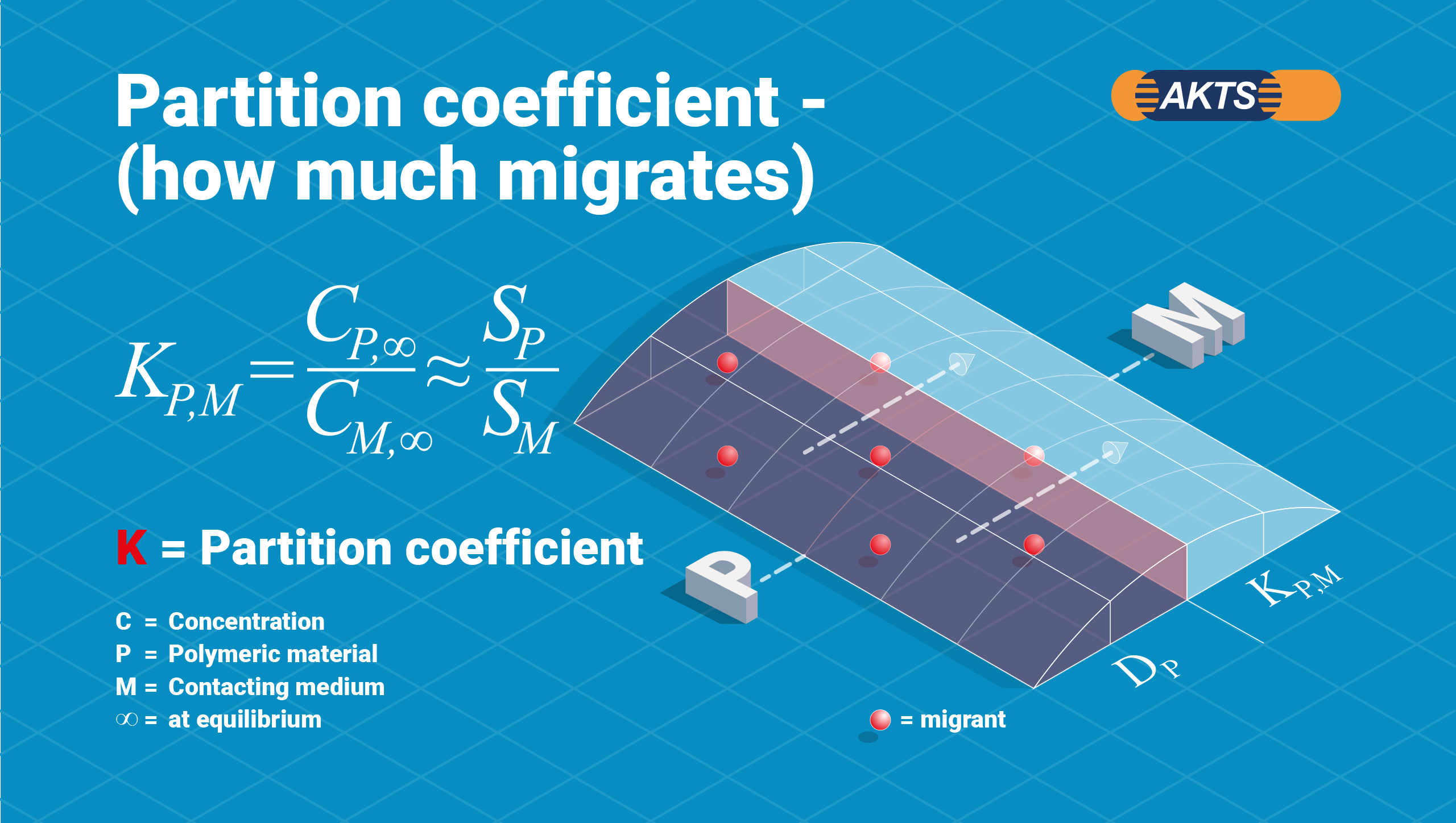
Fig. 5 – Partition coefficient
For the estimation of diffusion- and partition coefficients there are several scientific approaches:
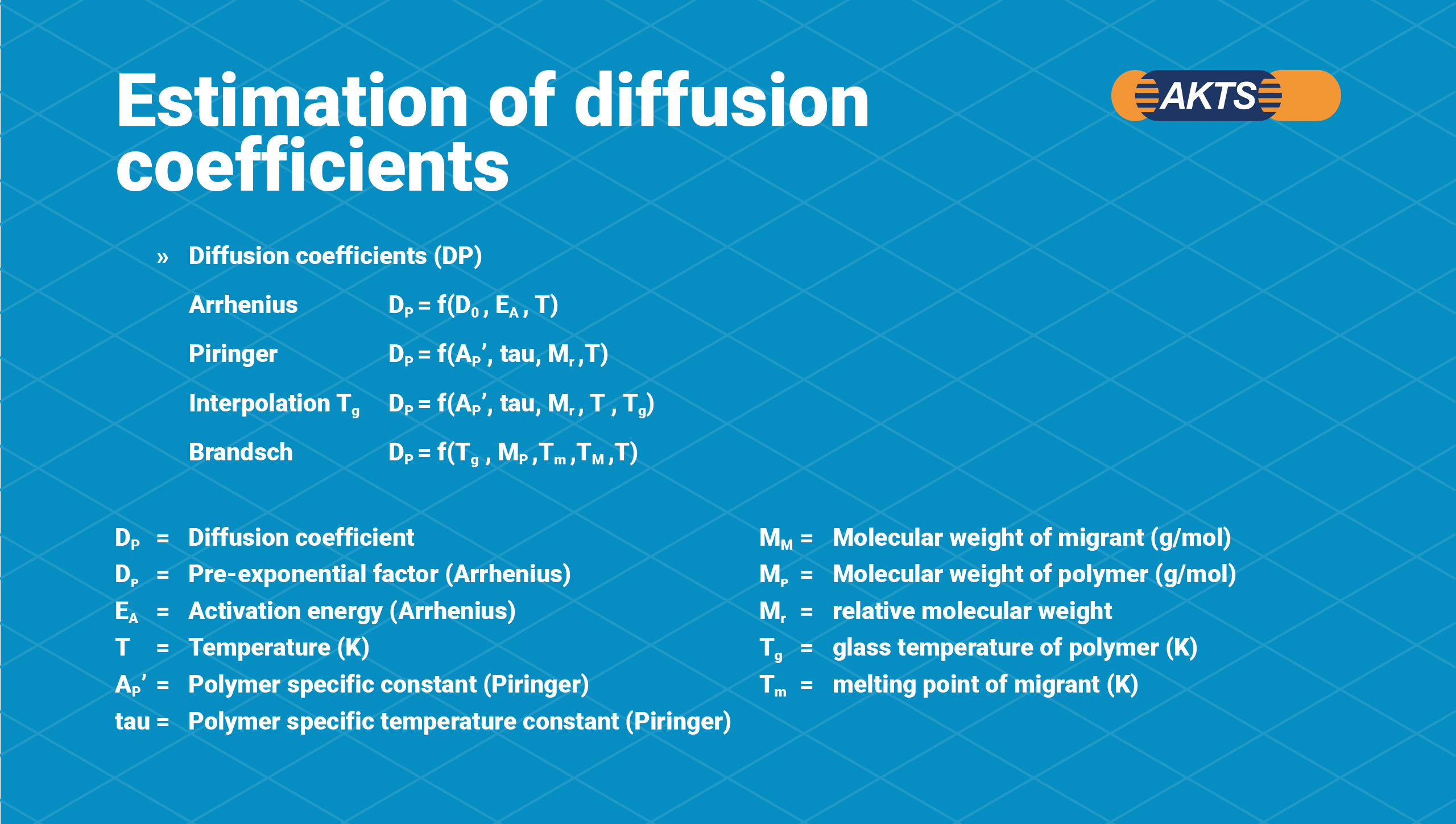
Fig. 6 – Methods of estimation of diffusion coefficients
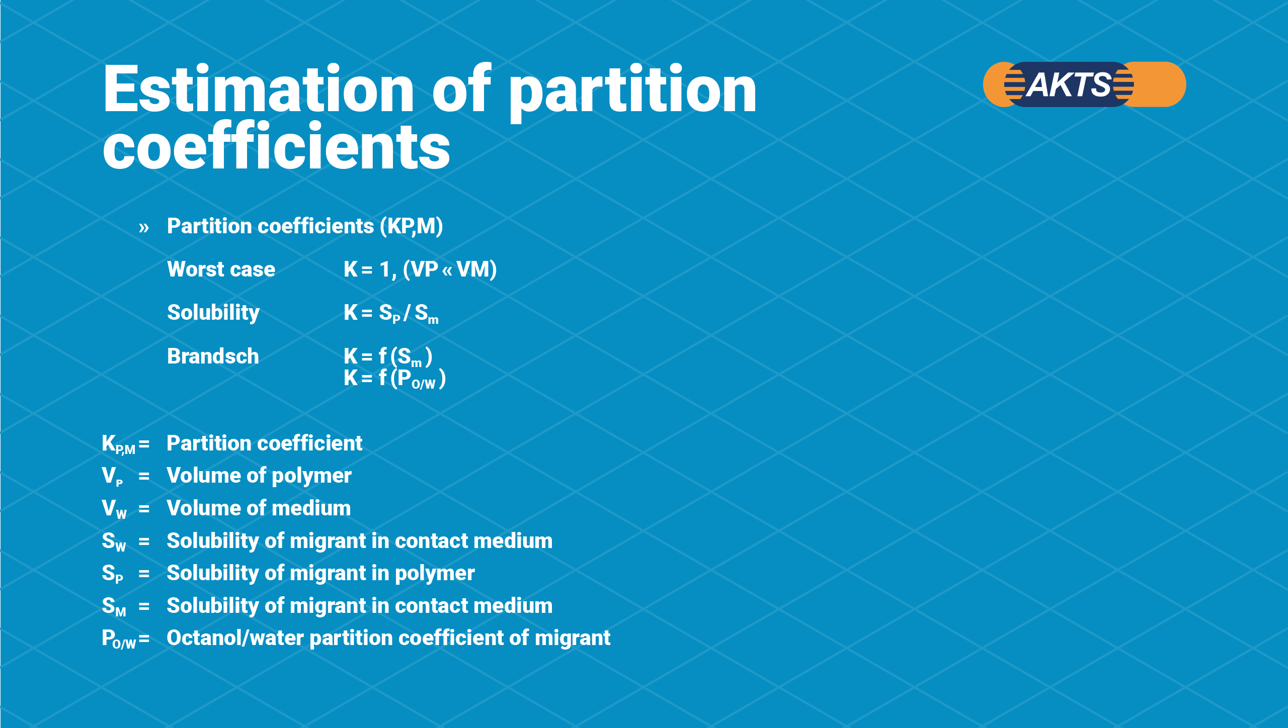
Fig. 7 – Methods of estimation of partition coefficients
For the estimation of diffusion coefficients according to Arrhenius and Piringer the experimental testing is required to determine material specific parameters like the pre-exponential factor D0; the activation energy EA; the polymer specific constant, AP and the polymer specific temperature constant, tau which corresponds to the deviation from the reference activation energy, EA=EA,ref+τ•R with R the gas constant. The influence of the migrant molecule structure on the diffusion rate may be considered by its molecular weight. The AP-value concept of Piringer was validated in the frame of an EU-project and confirmed by modelling of the migration from plastics into food simulants (polymeric material in contact with liquids).
The estimation of diffusion coefficients according to Brandsch is based on the application of the glass temperature of polymeric materials.
The procedure of the estimation of partition coefficients is less advanced. Nevertheless some scientific approaches exist based on a method developed by Piringer or an empirical approach developed by Brandsch in the frame of the EU-project “Foodmigrosure” [3].
The empirical approach by Brandsch considers the polarity of the migrant expressed by its octanol/water partition coefficients and sets it in relation to the partition coefficient between polymeric materials and real foods or food simulants.
AP value concept (Piringer)
The estimation procedure for diffusion coefficients according to Piringer, the so called AP-value concept, requires the experimental determination of the polymer specific constant, AP and the polymer specific temperature constant tau once for each polymer type. For each polymer the time dependent migration experiments must be run at different temperatures what allows the determination of the diffusion coefficients which, in turn, are used for evaluation of AP-values according to the relationship developed by Piringer. From all available AP-values an upper limit value for certain polymer material is calculated as the 95-percentile of that data set.
Experimental time dependent migration data, diffusion coefficients and AP-values are collected and evaluated by the Modelling Task Force at the Joint Research Centre of the EU-Commission.
For most of the polymeric materials used in food contact materials upper limit AP*-values and tau-values are listed in the JRC-Guideline supporting the Plastics Regulation (EU) No 10/2011 of the EU-Commission. Upper limit AP*-values result in overestimated migration values in support of consumer safety.
Overestimation and consumer protection
It is in support of consumer safety to develop procedures for estimation of mass transfer constants which systematically overestimate the migration behaviour of real polymeric materials. Due to systematic overestimation the risk of underestimation compared to the real system is minimized.
Due to simulation of one single migration cycle it is easy for food contact materials to implement overestimation. The use of upper limit AP-values in the estimation procedure of diffusion coefficients and lower limit partition coefficients results in estimated migration value which are higher compared to the real ones.
Repeated use
Polymer materials with repeated use or dynamic flow behavior of the contacting medium need more specific considerations. The experimental conventional test conditions as well as migration simulations account for the repeated use or dynamic flow behavior by implementation of several migration test cycles. Overestimating the migration in the first migration cycle may cause underestimation in later migration cycles. This can happen only if the overestimation based on diffusion and partitioning is very high and more than 50% of the migrant migrates out of the polymer in the first migration cycle. In these special cases, which can be easily identified during simulation, only the first migration cycle can be used for comparison with a specific migration limit.
[1] EU-project “Recyclability” FAIR-CT98-4318
[2] EU-project “Certified Reference Materials” G6RT-CT2000-00411
[3] EU-project “FOODMIGROSURE” QLK1-CT2002-2390
[4] EU-project “MIGRESIVES” COLL-CT-2006-030309
Legal background
Use of simulation (introduction)
Polymer materials are used in a variety of applications, see list below. In each case the consumer, directly or indirectly, may be exposed to the migrants (chemicals) present in polymers.
- Food contact materials and articles
- Toys
- Textiles
- Child and care articles
- Medical devices
- Drinking water pipes, bottles and containers
- Household articles
- Consumer goods
- Construction materials
- Automotive applications
- Electronics applications
- Other materials and articles
The legal requirements are set at national and international level for the evaluation of the acceptable migration level of the chemicals from plastics. For given applications like food contact materials or toys detailed legal requirements in terms of substance specific migration limits are set by the applicable legislation. Historically, the experimental approach, i.e. the experimental migration testing under conventional test conditions was used for compliance assessment.
Migration modelling is a valuable tool to estimate the type and extend of interaction between polymeric materials and contacting media. Estimating the mass transfer based on the relevant physical and chemical parameters as e.g. the mass transfer constants, enables evaluation of the migrants level at all stages of the production chain.
In the last years migration modelling is more and more accepted and it was first introduced in legislation for plastic food contact materials and articles in 2001 allowing for compliance assessment with applicable legislation.
Food contact materials
EU legislation
Migration modelling was introduced in the EU legislation for materials and articles intended to contact food with the 6. Amendment of Directive 90/128/EEC, today consolidated in Directive 2002/72/EC. The consolidated Plastics Directive 2002/72/EC was amended several times and finally repealed by Regulation(EU) No 10/2011 in May 2011.
Detailed information about the application of the generally recognized diffusion models can be found in the JRC Scientific and Technical Report, 2010; C. Simoneau, ed., “Application of generally recognized diffusion models for the estimation of specific migration in support of EU Directive 2002/72/EC.”
In the new Regulation (EU) No 10/2011 the Migration Modeling approach was defined in Annex V as one of the so called “screening approaches” which can be used in support of compliance evaluation for food contact plastics. The Plastics Regulation states: “To screen for specific migration the migration potential can be calculated based on the residual content of the migrant in the material or article applying generally recognized diffusion models based on scientific evidence that are constructed such as to overestimate real migration.”
According to Article 18 of Regulation (EU) No 10/2011 the migration modelling can be used to demonstrate compliance of food contact materials and articles with the applicable legislation. To demonstrate noncompliance, i.e. by official control, the experimental approach is compulsory.
Drinking water contact materials
German Recommendation
The German Recommendation “Leitlinie zur mathematischen Abschätzung der Migration von Einzelstoffen aus organi-schen Materialien in das Trinkwasser (Modellierungsleitlinie)” as of 7. October 2008 states:
The mathematical estimation of migration can be used to evaluate the compliance with requirements of the “KTW-Leitlinie”, “Beschichtungsleitlinie” or the “Schmierstoffleitlinie” regarding individual migrants instead of an experimental proof.
Other applications
Strong efforts are made to get migration modelling accepted for all applications where polymeric materials are used.
Because interaction between plastic materials and contacting media, i.e. migration and emission processes follow the same laws independently of the application one can expect that this objective will be achieved in near future.
For organic materials in contact with drinking water this objective was reached with introduction of the migration modeling approach by the German Umweltbundesamt with the “Modelierungsleitlinie”.
The Mathematical Model Applied for the Simulation of the Diffusion
Introduction
Some of existing computer programs are available to predict, for consumer protection purposes, the migration of additives from a polymeric material or article during its contact with food. However most of them were developed to estimate migration only from single layer polymeric packaging under isothermal conditions. In our SML Software a diffusion model was developed to simulate the migration from multilayer packaging and under any, arbitrarily chosen temperature mode.
General description of the model
Simulation of the diffusion processes of migrant and simulant occurring in packaging multi layers can be reduced to the analysis of a single layer.
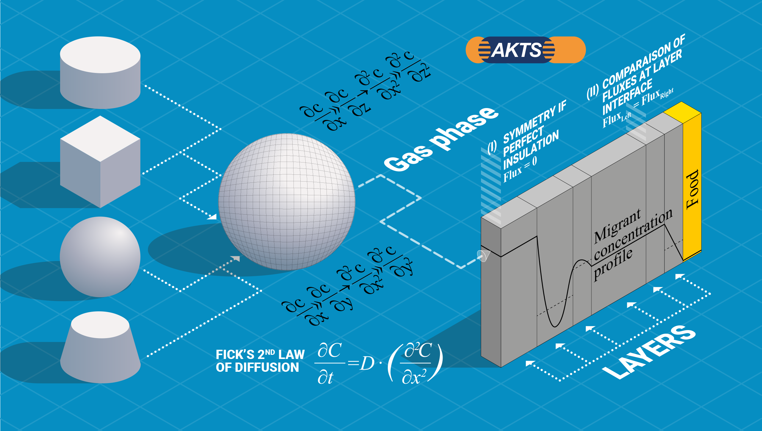
Fig. 1 – Scheme of the simulation of the migrant concentration in packaging
Considering one layer inside the packaging, it can be demonstrated that the mass of the layer which is taken for calculation of the diffusion of both, migrant and simulant, can be treated as an “infinite” surface of thickness “d” (i.e. “infinite” in two directions and of wall thickness “d” in the third). To calculate the amount of the migrant that reaches the food after a certain time all package geometries are reduced to a simple case: a plane of several sheets with only one surface in contact with the food. It can be assumed that diffusion obeys Fick’s law and that the diffusion of the species in the y and z direction is negligible as compared to x direction. The presented model enables calculations of the concentration gradients using numerical analysis methods, considering the diffusion progresses of both species (migrant and simulant) in the multi-layers. The Arrhenius, Piringer and Brandsch equations can be applied in order to evaluate a magnitude for the diffusion coefficient in the different layers. The equations have been developed using coordinates (x and t) where the whole surface of the packaging will be derived from the different packaging shapes.
Concentration distribution in the layers
Generalized mass balance over a layer volume element
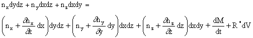
In order to consider the change of the concentration of the migrant (and/or simulant) diffusing inside the layer, a mass balance over a volume element can be made as following:
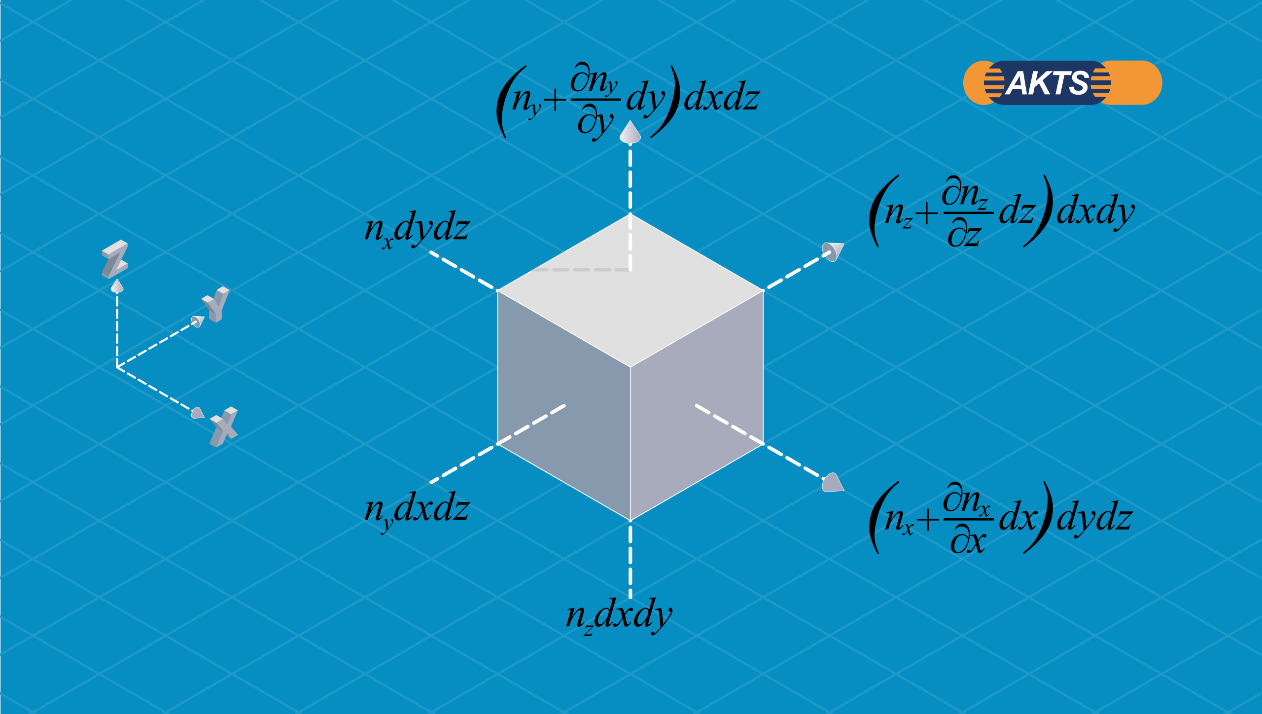
Fig. 2 – Generalized mass balance over a layer volume element
Input = Output + Accumulation + Reaction
 (2.1)
(2.1)
![]() (2.2)
(2.2)
![]() (2.3)
(2.3)
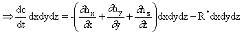 (2.4)
(2.4)
where
![]() (2.5)
(2.5)
 (2.6)
(2.6)
Considering cylindrical coordinates and generalizing the above equation we can write for a recipient
![]() (2.7)
(2.7)
![]() (2.8)
(2.8)
where J is a geometry factor which is dependent on the type of recipient:
J=0 for the infinite plate
J=1 for the infinite cylinder
J=2 for the sphere
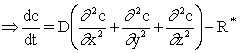
Without chemical reaction
![]() (2.9)
(2.9)
the mass balance for a migrant ‘M’ reads for an infinite plate:
![]() (2.10)
(2.10)
Similarly, the mass balance for a simulant S’ reads:
![]() (2.11)
(2.11)
with the following possible boundary conditions:
– Boundary (I): Symmetry axis (if perfect insulation):
![]() (2.12)
(2.12)
If a layer is insulated on its left or right side, the boundary condition is derived from the symmetrical properties of the concentration distribution at the wall surface of a layer U.
– Boundary (II): Considering the “left” and “right” sides of one interface, we can write at the interface between two layers U and U+1.
 (2.13)
This boundary condition is derived from comparison of fluxes at the interface between the different layers.
In the above scheme, the initial concentration of the migrant and solubility have to be set for each layer. To solve the problem we essentially apply the equation (2.8) under consideration of the boundary conditions. The solubility in each layer to “control” the effect of the partition coefficient at the interface between two layers is also considered in the calculation procedure. A mass balance can be established similarly for both, migrant and/or simulant.
Discretization of the layer domain
The packaging mass which is taken for the diffusion expressions can be treated as an “infinite” surface of thickness “d” (i.e. infinite in two directions -y, z directions- and of layer thickness “d” in the third -x direction-).
Using the generalized mass balance eq. 2.8 over one layer element in the packaging wall, we can relate the diffusion of e.g. a migrant ‘M’ in each layer. The scheme of the grid-point distribution applied for calculating the concentration distribution in each layer is presented below.
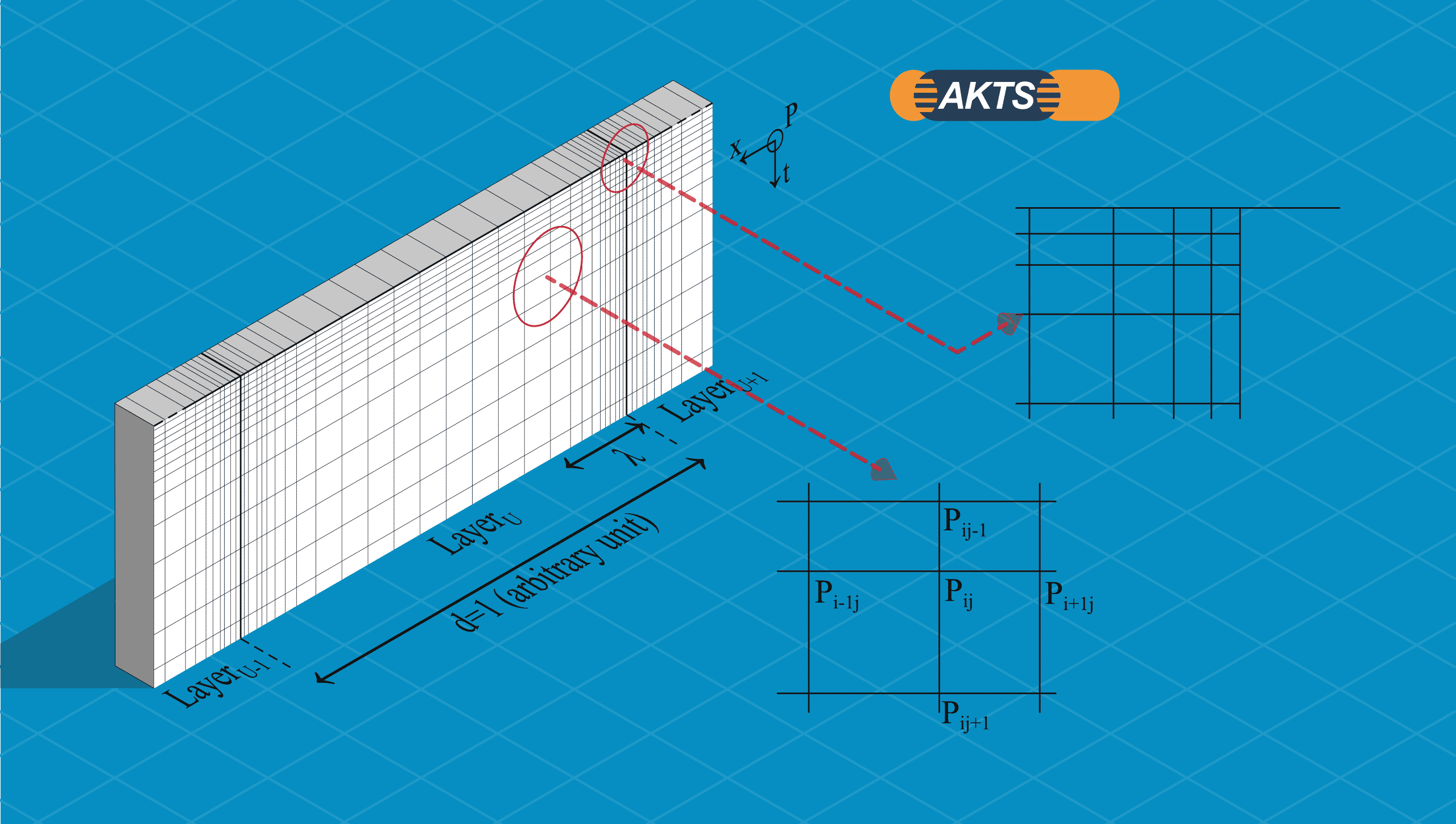
Fig. 3 – Description of a Layer “Domain”. The grid-point distribution is chosen with variable step lengths in the diffusion direction x as well as in time
The functions of the mass balance (eq. 2.8) are singular at the interface of the different layers and at the beginning of the diffusion process (times around 0). Therefore the grid-point distribution must be chosen with variable step lengths (see Fig. 2.3). The generation of adaptive meshes allows the achievement of a desired resolution in localized regions and decreases by orders of magnitude the calculation time. Grid points are added in regions of high gradients to generate a denser mesh in that region and subtracted from regions where the solution is decaying or flattening out.
The Fig. 4 illustrates the discretization of the governing partial differential eq. 2.8 describing the diffusion processes occurring inside the layer. The layers can be divided into a series of N mesh planes each having IxJ elements. The position of the mesh planes is moved along the time-axis allowing the calculation of the concentrations of both species (migrant and stimulant) at each location for every x, t grid points of each layer.
Discretization: Let us choose “n” for satisfying following conditions:
![]() (2.14)
(2.14)
![]() (2.15)
(2.15)
where λ = 1
e.g. λ = 1
describes with arbitrary units the length of a desired thickness inside one layer. After computing a series expansion of the above equations with respect to the variable “k”, we obtain:
![]() (2.16)
(2.16)
![]() (2.17)
(2.17)
Taking the natural logarithm, we can solve the inequality 2.17 for “n” and round the obtained value to the nearest integers towards minus infinity:
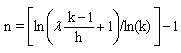 (2.18)
The concentration profile for the migrant may now be expressed by substituting finite-difference approximations. Taylor series expansions of the second derivates are computed, with respect to the variable x, up to the order three. The series data structure represents an expression as a truncated series in one indeterminate node, expanded about the particular point (i ,j) (see Fig. 2.3). The more detailed presentation of analysis is upon the scope of this help.
Programming
Using the boundary conditions expressed by eqs. 2.12-13 and eq. 2.8 which describes the diffusion in the bulk, the concentration distribution inside all layers can be computed for both migrant and the simulant. The initial concentrations of the migrant (in mg/kg units) have to be introduced for all layers at t = 0. The strong internal gradients are calculated very precisely due to the variable step lengths.
AKTS - SML Software
Software Basics
The use of AKTS-SML software can be described in four steps:

Fig. 4 – Applications of SML-Software from packaging definition to legislation conformity.
1. Define the package by creating the different articles of the package and introducing their properties.
2. Predict the migration using different temperature profiles (iso, non-iso, worldwide climate, etc.).
3. Analyze the calculated outputs.
4. Check the conformity of the results with corresponding legislations.
Package Structure
A package is a group of different articles, each having different layers properties. For instance a bottle can be treated as two articles: the bottle cap and the bottle body.

Fig. 5 – A package can be composed of multiple articles.
An article is composed of one or more layers of different sizes and properties.

Fig. 6 – An article is composed of multiple layers and Fig. 3.4 : Migrants can be found in all layers.
Chemicals can be found in one or more layers.
Creating packages and articles
The package details will be displayed by clicking on New Package.
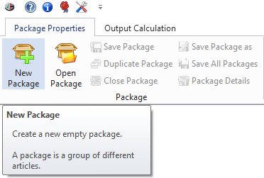
Fig. 7 – Creating a new package.
The Package Properties tab allows changing the geometry and the size of the package. The surface, shape and size of each article can be defined in the grid.

Fig. 8 – The package panel for packaging and article creation.
The Wizard
When creating an article, many information and properties have to be implemented. The role of the Article Creation Wizard is to help introducing all this information step by step.
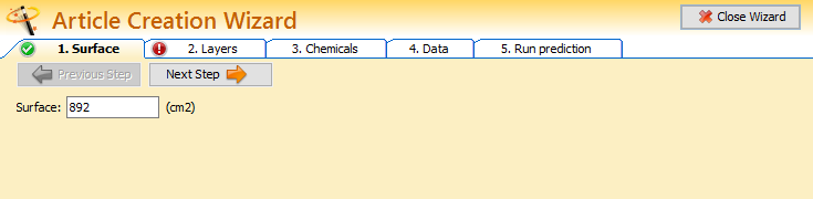
Fig. 9 – The wizard interface.
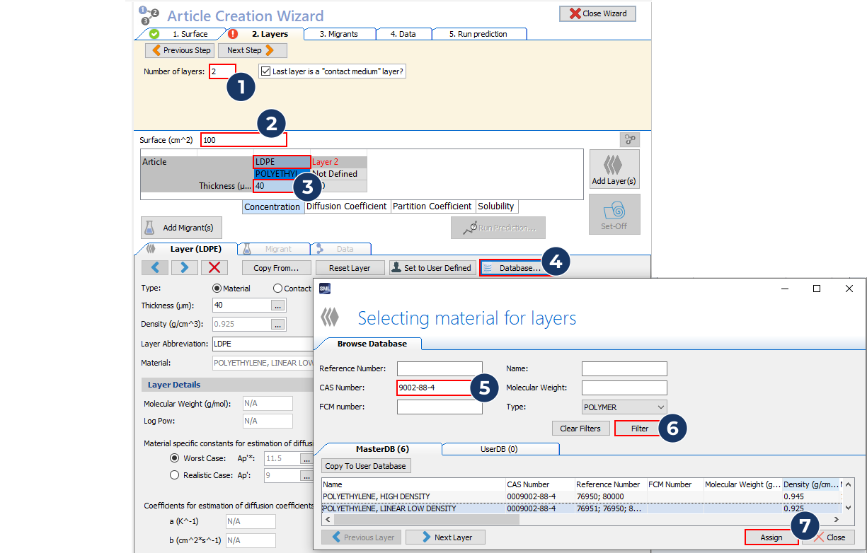
1. Surface: The surface of the article has to be entered first.
2. Layers: Then enter the number of layers and give the information for each of them.
3. Migrants: Enter the number of chemicals and fill the information for each of them.
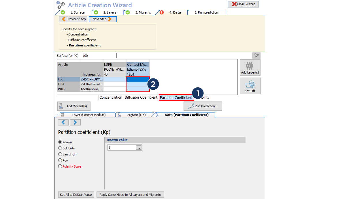
4. Data: First specify the concentration of each migrant in each layer, then the diffusion coefficients and finally the partition coefficient.
When the package data are fully implemented, it is possible to start calculating predictions by clicking on the Run Prediction button
Note: the Wizard is optional.
Article Properties
The article grid.

Fig. 10 – The article grid.
In the Article Grid it is possible to customize the concentration, the diffusion coefficient and the partition coefficient for all migrants and layers.
The button Add Layer adds a new layer displayed as a column in the grid.
The button Add Migrant(s) adds a new chemical displayed in a row in the grid.
See more about:
- The layer properties;
- The migrant(s) properties;
- The data (concentration and coefficients).
When all the properties of the article are introduced click on Run Prediction to start a calculation process. See the Predictions chapter for more information.
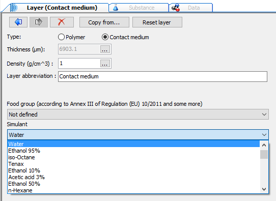
Layers
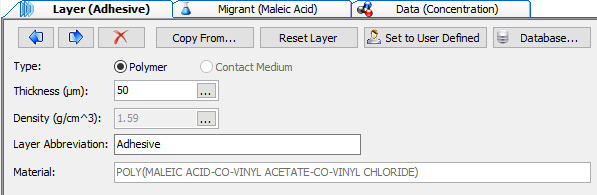
Fig. 11 – Layer properties.
The layer properties panel allows defining the properties of the current selected layer.
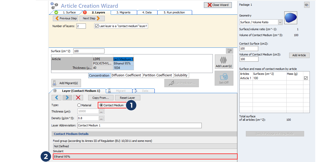
Type (of layer) defines if the layer is a contact medium (typically food) or a polymer.

Fig. 12 – Considered Properties of Polymer Type Layer.
Database allows browsing for a known polymer.
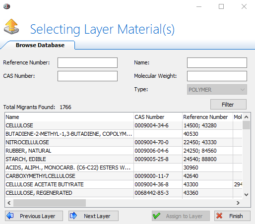
Fig. 13 – Layer Material(s) Database.
Contact medium
Set to user defined allows customizing the properties of the polymer.
When the polymer is set to user defined, it is possible to enter manually the properties of the polymer. Otherwise, if the polymer is loaded from the database, its properties are filled automatically.
Reset layer allows setting the default values.
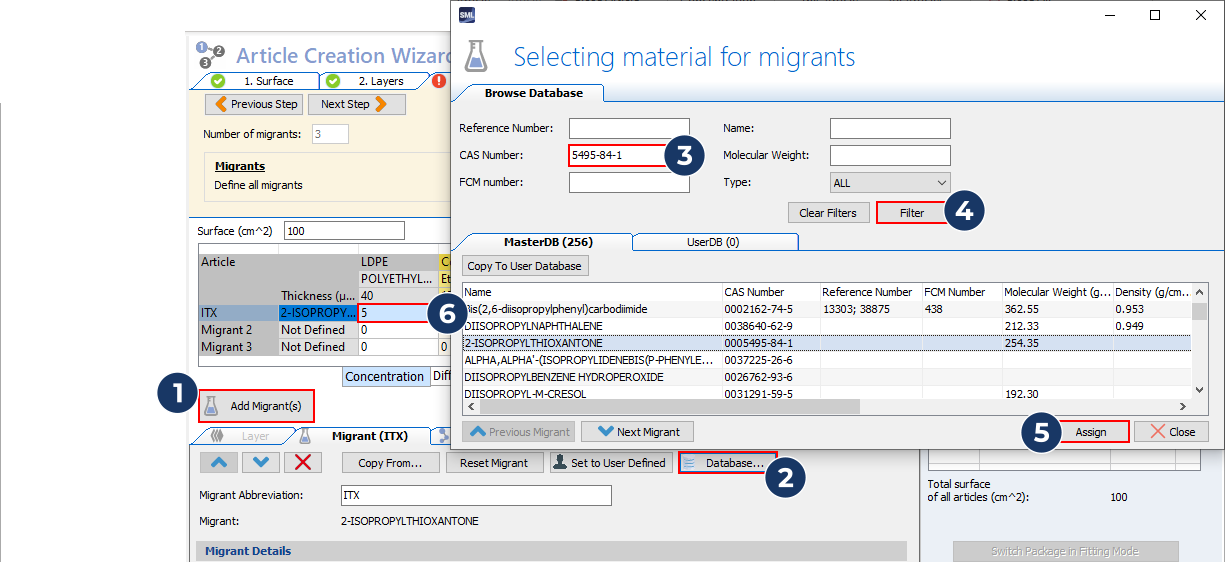
Migrants properties
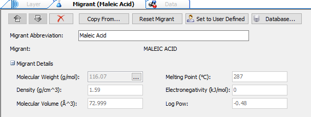
Fig. 16 – Considered Migrant Properties
The migrant properties panel allows defining the properties of the currently selected migrant. When the migrant is set as user defined, it is possible to enter manually its properties. Otherwise, if the migrant is loaded from the database, its properties are filled automatically.
Database allows browsing for known migrants (more than 20000 chemicals: additives, monomers, photo initiators, pigments, solvents, etc.).
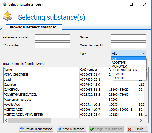
Fig. 17 – Migrant database
Data concentration, diffusion and partition coefficients
The Data tab allows defining:
- the concentration;
- the diffusion coefficient;
- the partition coefficient.
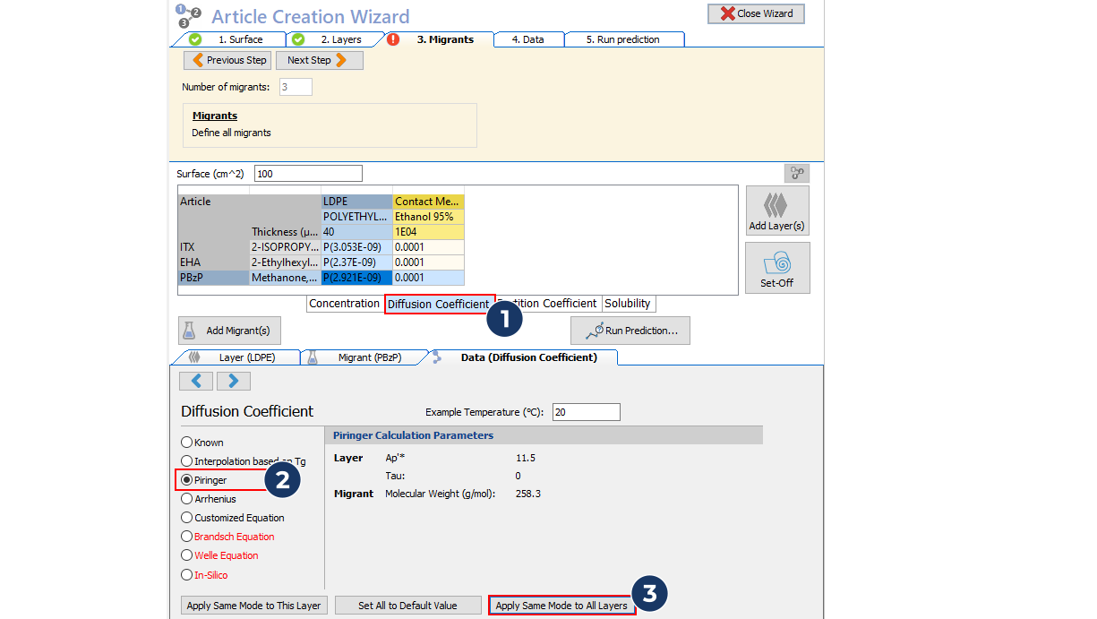
Diffusion coefficient
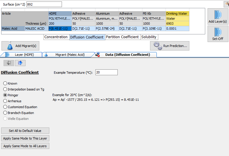
Fig. 18 – Determination of the Diffusion Coefficients. The Data Properties shown are based on the currently selected tab of the article grid.
The diffusion coefficient values can be entered manually when known, or it is possible to load the values from the database, to use an Arrhenius, Piringer or Brandsch calculation methods or apply a customized equation.
Piringer Model
Piringer model estimates diffusion coefficients for migrants in polymers from Ap-value of polymer and molecular weight of migrant by use of a fixed activation energy based on Arrhenius type equation. It is considered that the Piringer model is fully validated for some basic polymers see Guideline. More about the wording validated: a given polymer types as e.g. PE is considered to be fully validated according to the Guideline if an upper limit Ap*-value can be established with sufficient statistical certainty and assures that in 95% of all cases for any PE on the market for any migrant of interest at any temperature the real migration behavior is overestimated. It is a long way to generate sufficient experimental migration kinetics data to claim that a polymer is fully validated. The drawback of a validated upper limit Ap*-value is that they include any scattering from the polymer under investigation (many different grades on the market), scattering from experimental migration kinetics (experimental setup or analytical problems), scattering induced by Piringers formula (assumes a fixed activation energy for diffusion), and some more sources of uncertainty. As a consequence diffusion coefficients estimated with fully validated upper limit Ap*-values are overestimated (in most cases significantly) compared to real diffusion coefficients. In fact validated upper limit Ap*-values are useful only for assessment of compliance with SML-values. To model realistic migration more realistic Ap*-values and respectively, diffusion coefficients should be used. These can be taken from literature or more refined estimation procedures like using the realisti Ap*-values, i.e. the mean value of the distribution.
Brandsch Equation
Brandsch equation is based on Arrhenius relationship but on completely different approach compared to Piringer. Required inputs are the molecular weight of the migrant and of the polymer, the melting point of the migrant and the Tg of the polymer. Main difference to Piringers approach is, that Brandsch equation applies a variable activation energy in dependence on the migrant size (expressed by its molar volume). The Brandsch equation gives a reasonable from the scratch estimate for diffusion coefficients in polymers for which a Tg is available or can be determined experimentally. The Brandsch equation is an option to be taken for situations were no other option to estimate diffusion coefficients is available.
Remarks
- Case of PVC: According to Modelling Guideline Piringer approach is validated only for molecules with molar mass > 225 g/mol. As a result, the Piringer approach is underestimating migration for small molecules, especially if no experimental migration data were available for validation as in the case for PVC. In this case the Brandsch equation accounts for the small molar mass and the very low melting point (high volatility) of the molecule.
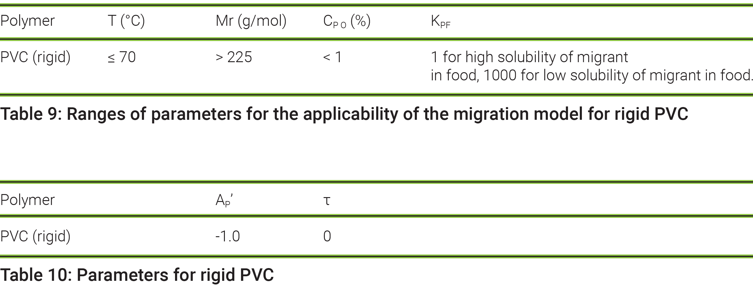
- Please note that to perform a migration modelling calculation with SML software you don’t need to select a polymer from the database, but make the inputs for the polymer in the user defined mode. Please make an input for the glass transition temperature of your polymer under investigation. Then for estimation of the diffusion coefficient you can select interpolation by Tg.
- Please consider that Ap-values (and any other estimation procedures for diffusion coefficients) are based on experimental data e.g. migration kinetics investigated under defined time/temperature/simulant conditions. It means that the models are as good as the quality of experimental data available.
- The estimation procedures in the SML software reflect the actual state of knowledge regarding diffusion properties of polymers. If new high quality experimental data become available, estimation procedures will become more precise. Due to scattering of experimental data for the use of migration modelling for compliance purpose, i.e. simulation of specific migration, the upper limit concept was introduced due to which migration by modelling is overestimated (sometimes strongly) compared to the real migration behavior.
- Provided the solubility of the migrant in the simulant is compelling, the diffusion coefficients can be extracted from single point migration results. This option is less precise, i.e. will cause significant scattering of the data, but should help understanding diffusion properties of concerned plastics.
- It is up to industry to decide whether they want to continue testing single SML results and waste their money or they want to join forces to develop diffusion models for their plastic materials. In long term, to our opinion, in the EU, the second option will be more cost effective.
- Comparison of modelling calculation with experimental results should be done very carefully. Experimental results may not be correct if they are produced under conditions which cannot be compared with modelling calculations, e.g. testing PET with ethanol simulant which causes swelling of the PET and change its diffusion properties.
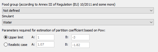
Partition coefficient
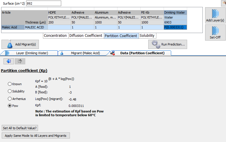
Predictions for different temperature profiles
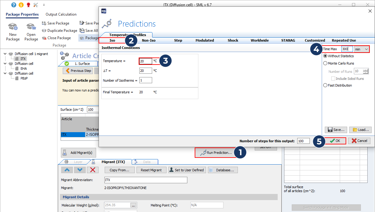
When all properties of an article are introduced, it is possible to proceed with prediction calculations by clicking on the Run Prediction button.
![]()
Fig. 20 – The run prediction button
The predictions can be performed for different temperature profiles:
- Isothermal
- Non-Isothermal
- Stepwise
- Modulated
- Shock
- Worldwide
- STANAG
- Customized
Isothermal
In the isothermal conditions mode, it is possible to set a number of isotherms and the temperature difference (ΔT) between each isotherm.
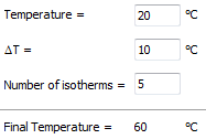
Fig. 21 – Isothermal conditions
Non-Isothermal
In the non-isothermal conditions, the starting temperature and different heating rates can be defined.
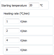
Fig. 22 – Non-Isothermal conditions
Stepwise
The stepwise conditions are a combination between isothermal and non-isothermal temperature modes. A number of cycles can be defined.

Fig. 23 – Stepwise conditions
Modulated
In the modulated conditions, it is possible to set an oscillatory temperature mode as e.g. a day/night cycle

Fig. 24 – Modulated conditions
Shock
The shock temperature conditions simulate a rapid temperature raise. The frequency of the temperature shocks can be also defined.
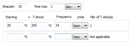
Fig. 25 – Shock conditions
Worldwide
The worldwide temperature mode allows calculating predictions for real atmospheric temperatures. The temperatures can be chosen for different climates (yearly temperature profiles with daily minimal and maximal fluctuations).
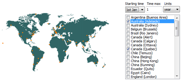
Fig. 26 – Worldwide conditions
STANAG
STANAG 2895 is a NATO Standardisation Agreement describing the principal climatic factors which constitute the distinctive climatic environments found throughout the world.
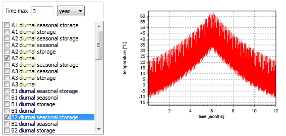
Fig. 27 – STANAG conditions
Customized
The customized prediction mode allows loading a file with a custom temperature profile, e.g. collected by a data logger.

Fig. 28 – Customized conditions
Outputs
The output window shows the results of the prediction calculations. The window is divided as following:
- The results grid;
- The c(t) chart;
- The c(x, t) chart;
- Comparison Output;
- Sum Output
Moving the mouse pointer over the c(t) chart will update the results grid and the c(x, t) chart based on the time pointed on the c(t) chart.
The results grid
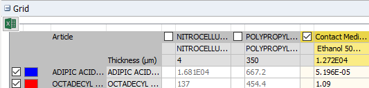
Fig. 29 – The Results Grid c(t)
The grid shows the values of the concentration, the diffusion coefficients and the partition coefficients for all migrants in all layers.
The c(t) chart
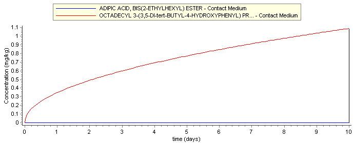
Fig. 30 – The c(t) chart
The c(t) chart shows the dependence of the concentration of the migrant as a function of time. The chemicals and layers to be displayed can be selected by using the checkboxes in the results grid.
Exportation and importation of c(t) and c(x,t) dependences for comparison can be done by a right-click on the calculated results as presented in the next figure.
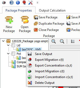
Fig. 31– Import / Export of c (t) Chart
The c(x, t) chart

Fig. 32 – The c(x, t) chart
The c(x, t) chart shows the spatial concentration of the migrant in the different layers.
Exportation and importation of c(t) and c(x,t) curves for comparison can be done by a right-click on the calculated results as presented in the next figure.
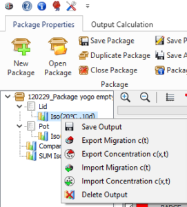
Fig. 33 – Import / Export of c (x, t) Chart
Comparison Output
The comparison output window allows comparing the calculation results of different outputs. To add an output to the comparison, drag and drop the output from the list on the left to the dedicated zone in the comparison output window.
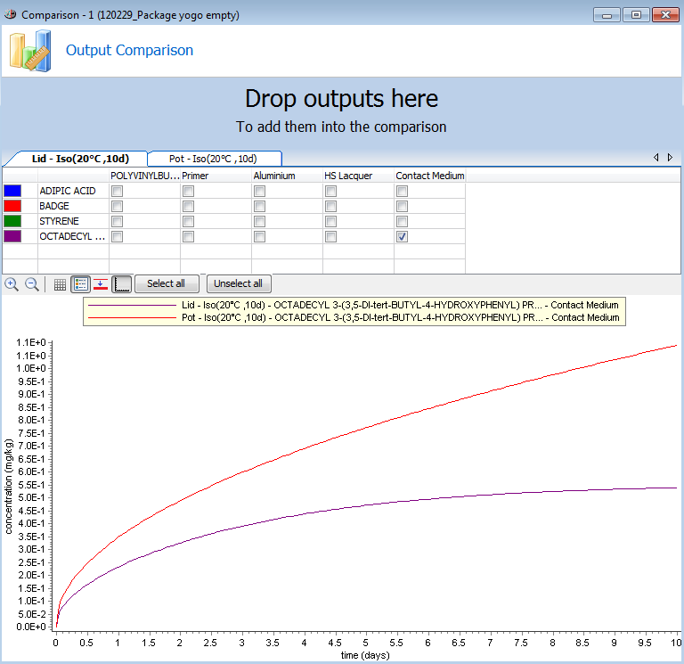
Fig. 34 – The comparison output window
Sum Output
The sum output window allows adding the calculation results presented in different outputs of same migrants. To add an output to the comparison, drag and drop the output from the list on the left to the dedicated zone in the comparison output window.
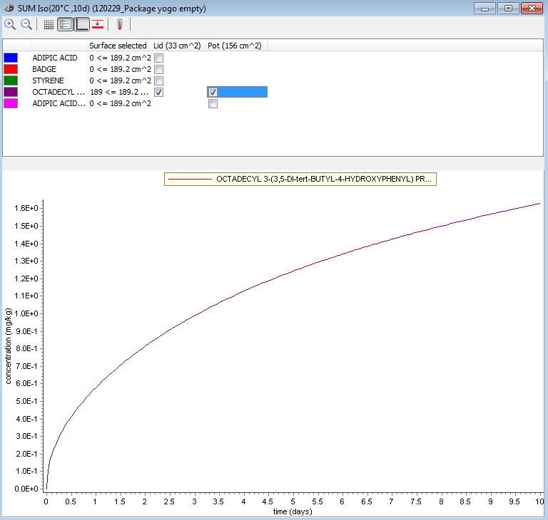
Fig. 35 – The sum output window
Legislation and compliance
Legislation conformity check: Compliance evaluation for substances with specific migration limit (SML) listed in the Plastics Regulation (EU) No 10/2011 and generation of compliance certificates.
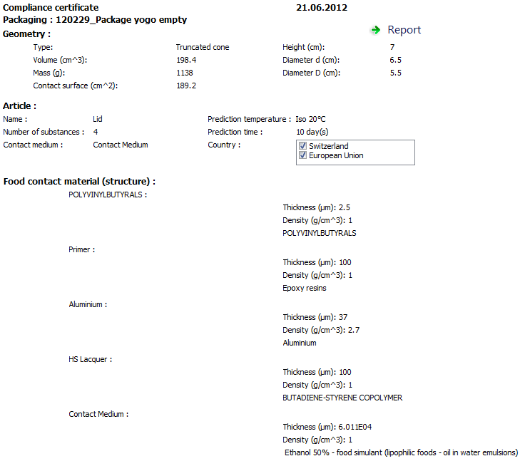
Fig. 36 – Legislation and compliance report (calculated migration values)
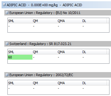
Fig. 37 – Legislation and compliance report (migration limits)
Sensitivity analysis methods
Introduction
Sensitivity analysis studies allow estimating how the uncertainties in the model inputs (X1;X2;…;Xk) affect the model’s response Y, which (for simplicity) we assume to be a scalar:
Y = f(X1;X2;…;Xk);
where f describes the implemented model.
A sensitivity analysis attempts to provide a ranking of the model’s input assumptions with respect to their contribution to model output variability or uncertainty. The difficulty of a sensitivity analysis increases when the underlying model is nonlinear, nonmonotonic or when the input parameters range over several orders of magnitude. Many sensitivity analysis methods have been proposed. For example, the partial rank correlation coefficient and standardized rank regression coefficient have been found to be useful. Scatter plots of the output for each of the model inputs can be a very effective tool for identifying sensitivities, especially when the relationships are nonlinear. In a broader sense, the sensitivity analysis can show how conclusions may change if models, data, or assessment assumptions are changed, see [1] for more details on the subject.
The analysis methods available in SML software are:
- Monte Carlo
- Fourier Amplitude Sensitivity Test (FAST)
- Sobol
Monte Carlo Simulation (MCS)
Monte Carlo Simulation (MCS) is a widely used method applied for uncertainty or sensitivity analysis. It involves random sampling from the distribution of inputs and successive model runs until the desired accuracy of the outputs is reached. Not only the means and variances but also the distributions of input parameters are required to run the MCS. In the present version of SML Software only Gaussian (normal) distribution has been implemented for the different input parameters.

Fig. 38 – Random sampling from the distribution of inputs (Gaussian (normal) distribution).
The main advantage of the MCS is its general applicability. MCS suffers for its computational requirements since thousands of repetitive runs of a model are required to reach convergence. High-speed personal computers have minimized the computational challenges. Another limitation of MCS is the need for user-specified rules for determining the number of simulations required, see [2-4] for more information and recommendation on the subject.
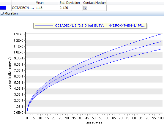
Fig. 39 – Quantification of the amount of variance that each input factor Xi (all variables of the articles) contributes with on the unconditional variance of the output V (Y).
Sensitivity measures based on the MCS approach include regression-based measures applying Standardized Regression Coefficients (SRC), Partial Correlation Coefficients (PCC), Standardized Rank Regression Coefficients (SRRC), Partial Rank Correlation Coefficients (PRCC). Some of them have been implemented in the present version of SML and are described below.
Correlation coefficient (CC) and partial correlation coefficients (PCC)
The correlation coefficient (CC) usually known as Pearson’s product moment correlation coefficients, provides a measure of the strength of the linear relationship between two variables x and y and is denoted as corr(x; y), see for example [5] for more information on the definition of CC.
The correlation coefficient measures the extent to which y can be approximated by a linear function of x, and vice versa. In particular if exactly y = a + bx, then corr(x; y) = 1, if b = 1 and corr(x; y) = -1, if b = -1. CC only measures the linear relationship between two variables without considering the effect that other possible variables might have. When more than one input factor is under consideration, as it usually is, the partial correlation coefficients (PCCs) can be used instead to provide a measure of the linear relationships between two variables when all linear effects of other variables are removed. PCC between an individual variable xi and y can be written in terms of correlation coefficients, see for example [5]. It is denoted by pcc(xi; y). PCC characterizes the strength of the linear relationship between two variables after a correction has been made for the linear effects of the other variables in the analyses.
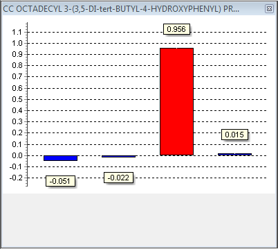
Fig. 40 – Correlation coefficients (CC) providing a measure of the strength of the linear relationship between two variables x (variable parameters in the article) and y (migration).
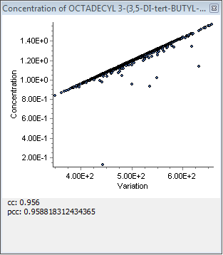
Fig. 41 – Scatter plots illustrating relationships between the input factor Xi (variable parameters in the article) and the output Y (migration).
A scatter plot of the points [Xij ; Yj ] for j = 1; 2;…;N can reveal nonlinear or other unexpected relationships between the input factor Xi and the output Y. Scatter plots are undoubtedly the simplest sensitivity analysis technique and their applications is a natural starting point in the analysis of a complex model. It facilitates the understanding of model behavior and the planning of more sophisticated sensitivity analysis.
Rank correlation coefficient (RCC) and partial rank correlation coefficients (PRCC)
Since the use of the correlation coefficient and partial rank correlation coefficient methods is based on the assumption of linear relationships between the input-output factors, they will perform poorly if the relationships are nonlinear. The SML-Software allows applying the rank transformation of the data. This concept can be used to transform a nonlinear but monotonic relationship to a linear relationship. When using rank transformation the data are replaced with their corresponding ranks. The usual correlation procedures are then performed on the ranks instead of the original data. Spearman rank correlation coefficient (RCC) is the corresponding CC calculated on ranks and partial rank correlation coefficients (PRCC) is the PCC calculated on ranks.
Rank transformed statistics is more robust, and provides a useful solution in the presence of long tailed input-output distributions. A rank transformed model is not only more linear, it is also more additive. Thus the relative weight of the first-order terms is increased on the expense of higher-order terms and interactions, see for example [5].
Variance based methods for sensitivity analysis
The main idea of the variance-based methods is to quantify the amount of variance that each input factor Xi contributes with on the unconditional variance of the output V (Y).
We are considering the model function: Y = f(X), where Y is the output and X = (X1;X2;…;Xk) are k independent input factors, each one varying over its own probability density function. The values of the input parameters are not exactly known. We assume that this uncertainty can be handled by using random variables Xj , j = 1;…; k of known distributions. Then the model output is also a random variable Y = f(X1; : : : ;Xk).
The first order effect for the input factor j is the fraction of the variance of the output Y which can be attributed to the input Xj and is denoted by Sj , see for example [5].
To estimate the value of Sj we require realizations of the input distributions and the associated model evaluations. The ratio Si was named as a first order sensitivity index by Sobol [6]. The first order sensitivity index measures only the main effect contribution of each input parameter on the output variance. It doesn’t take into account the interactions between input factors. Two factors are said to interact if their total effect on the output isn’t the sum of their first order effects. The effect of the interaction between two orthogonal factors Xi and Xj on the output Y can be computed (see for more details [5]) and is known as the second order effect. Higher-order effects can as well be computed, see for example [5].
A model without interactions is said to be additive, for example a linear one. The first order indices sums up to one in an additive model with orthogonal inputs. For additive models, the first order indices coincide with what can be obtained with regression methods. For non-additive models we would like to know information from all interactions as well as the first order effect. For non-linear models the sum of all first order indices can be very low.
The sum of all the order effects that a factor accounts for is called the ‘total’ effect [7]. So for an input Xi, the total sensitivity index STi is defined as the sum of all indices relating to Xi (first and higher order).
There are different techniques to obtain these sensitivity indices, such as Sobol’s indices, Jansen’s Winding Stairs technique, (Extended) Fourier Amplitude Sensitivity Test ((E)FAST).
In the present software, two methods are implemented, the FAST method and the Sobol’s indices based on Jansen’s Winding Stairs technique.
Fourier Amplitude Sensitivity Test (FAST)
The Fourier Amplitude Sensitivity Test (FAST) was proposed already in the 70’s [8-10] and was since this time successfully applied to chemical reaction systems involving sets of coupled, nonlinear rate equations.
FAST is a sensitivity analysis method which does not use a Gaussian distribution. Rotating vectors are assigned to each variable, and each has a unique frequency and the amplitude of the “mean”. A lot of input sets are generated, making the variables oscillating. A Fourier analysis is then applied on the results. The number of runs depends only on the number of variables.
Note that the graphs displaying the results obtained by the FAST method are the same as the graphs presenting results obtained with Sobol, approach except that FAST shows only the local sensitivity.
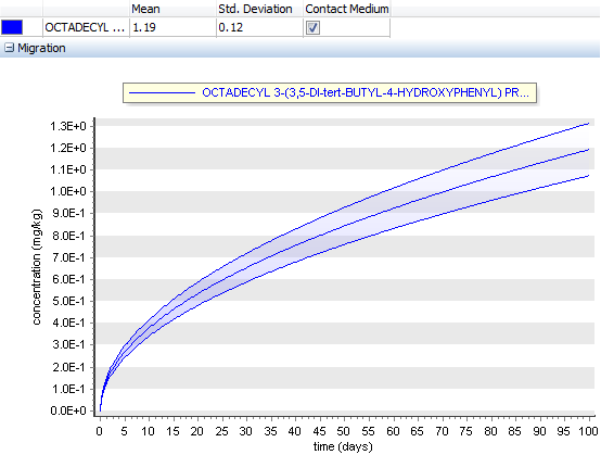
Fig. 42 – Quantification based on FAST analysis of the amount of variance that each input factor Xi (all variables of the articles) contributes with on the unconditional variance of the output V (Y).
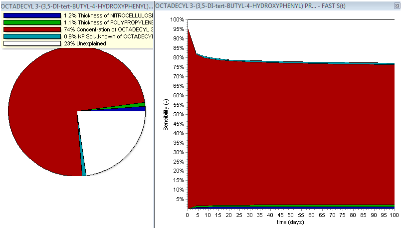
Fig. 43 – FAST analysis results. Sensitivity S(v) of each variable (influence of each examined variable on the migration results)
Sobol’s indices via Winding Stairs
Chan, Saltelli and Tarantola [11] proposed the use of a new sampling scheme to compute both first and total order sensitivity indices in only N x k model evaluations. The sampling method used to measure the main effect was called Winding Stairs, developed by Jansen, Rossing and Deemen in 1994 [12].
A first set of variables simply comes from the Gaussian distribution. Then a lot of other set of input of variables are generated from the first set and used in complex mathematics analysis afterward (For example: if one enters 10 runs and has one migrant with four variables, it will run the simulations (4+1)*10 times)
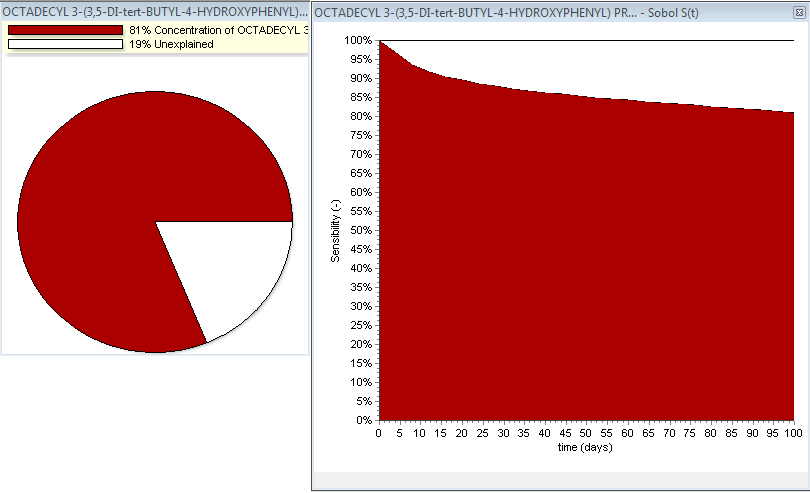
Fig. 44 – Sobol analysis results. Total sensitivity St(v) of the variables (influence of all variables on the migration results)
The above figures illustrate the total sensitivity St(v) of the variables (influence of all variables on the migration results) and the evolution of the total sensitivity as a function of time. In some cases there are “unexplained” values. This situation can happen when the calculation is not fully completed. Two cases are possible:
- The number of runs chosen to perform the calculations is not sufficient;
- Not enough variables are chosen to apply the method correctly.
Comments about our example :
All methods clearly demonstrate for our examined article that the initial concentration of the migrant (OCTADECYL 3-(3,5-DI-tert-BUTYL-4-HYDROXYPHENYL) PROPIONATE) plays the most important role concerning its migration from the article to the contact medium. The other parameters such as the thickness of both layers and the solubility of migrant in the contact medium have in comparison a negligible influence on the migration.
[1] A. Saltelli, K. Chan, M. Scott (Eds.). Sensitivity Analysis Probability and Statistics Series, John Wiley and Sons, 2000.
[2] J. C. Helton, F. J. Davis. Sampling Based Methods. Chapter 6 in Mathematical and Statistical Methods for Sensitivity Analysis of Model Output. Edited by A. Saltelli, K. Chan, and M. Scott, John Wiley and Sons, 2000.
[3] Helton J. C. Uncertainty and sensitivity analysis techniques for use in performance assessment for radioactive waste disposal. Reliability Engineering and System Safety, 42, 327 – 367, 1993.
[4] http://www.epa.gov/reg3hwmd/risk/human/info/guide1.htm
[5] P.-A. Ekström A simulation toolbox for sensitivity analysis, degree project, 2005.
[6] I. M. Sobol’. Sensitivity analysis for nonlinear mathematical models. Mathematical Modeling and Computational Experiment, 1, 407 – 414, 1993.
[7] T. Homma and A. Saltelli. Importance measure in global sensitivity analysis of nonlinear models. Reliability Engineering and System Safety, 52, 1 – 7, 1996.
[8] R. I. Cukier, C. M. Fortuin, Kurt E. Shuler, A. G. Petschek, and J. H. Schaibly. Study of the sensitivity of coupled reaction systems to uncertainties in rate coefficients. I theory. The Journal of Chemical Physics, 59, 3873 – 3878, 1973.
[9] J. H. Schaibly and Kurt E. Shuler. Study of the sensitivity of coupled reaction systems to uncertainties in rate coefficients. II applications. The Journal of Chemical Physics, 59, 3879 – 3888, 1973.
[10] R. I. Cukier, J. H. Schaibly, and Kurt E. Shuler. Study of the sensitivity of coupled reaction systems to uncertainties in rate coefficients. III analysis of the approximations. The Journal of Chemical Physics, 63, 1140 – 1149, 1975.
[11] Karen Chan, Andrea Saltelli, and Stefano Tarantola. Winding stairs: A sampling tool to compute sensitivity indices. Statistics and Computing, 10, 187 – 196, 2000.
[12] M.J.W. Jansen, W.A.H. Rossing, and R.A. Daamen. Monte Carlo estimation of uncertainty contributions from several independent multivariate sources. Predictability and Nonlinear Modelling in Natural Sciences and Economics, 334 – 343, 1994.
Repeated use
Introduction
Single use food contact materials like food packaging are in the focus of the food contact legislation. Repeated use food contact materials like kitchen utensils, drinking bottles, food processing equipment, etc. are as important. Generally, migration will reduce upon successive uses because the migration is determined by diffusion. Occasionally the migration may increase upon successive uses, e.g. migration of formaldehyde from phenol-formaldehyde or melamine-formaldehyde articles may increase due to hydrolysis in addition to diffusion. Therefore, migration from repeated use articles e.g. a food storage box or a bowl or plate should be assessed in three successive contact periods, using a new portion of food simulant for each contact period. Conventionally the migration found in the third migration experiments shall comply with the relevant specific migration limit.
Determination of the migration from a repeated use article does not deviate from the procedure followed for single use articles. However, establishing the right contact conditions of time and temperature as well as actual surface to volume ratio may be more complex. More details can be found in the guidelines of the EU Commission and the Joint Research Center:

Fig.45 – Guidelines on testing conditions for articles in contact with foodstuffs. Technical guidelines for compliance testing.
More complex repeated use scenarios are relevant for plastic materials in contact with drinking water. The migration simulation follows the testing requirements given in DIN EN 12873-1 and 2 and the KTW Guideline of the German UBA:
- cold water: 1 + 3 x 3 days;
- warm water: 1 + 3 x 1 + 3 + 3 x 1 days;
- hot water: 1 + 3 x 1 + 3 + 3 x 1 days.
According to the KTW Guideline of the German UBA extended testing cycles up to 31 days by repeating the above 10 days test cycles is optional but compulsory for multilayer materials.
The above-mentioned test cycles are implemented as predefined cycles in the SML 6 software:

Fig. 46 – Predefined cycles in the predictions window.
or can be customized by user by e.g. extending of testing scheme for 31 days = 4 x [4 x 1 + 3] + 3 x 1 d

Fig. 47 – Set up of an advanced repeated use function.
Example
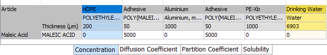
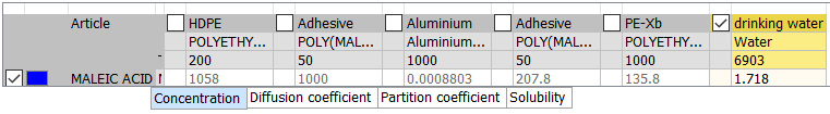
The application of the the repeated use function implemented in the SML 5.3 software is illustrated for the composite drinking water pipe with the layered structure HDPE/Aluminium/PE-Xb:

Fig. 48 – Composite drinking water pipe.
It is assumed that the adhesive layer between the plastic (HDPE and PE-Xb) and the Aluminum layers contains a residual amount of 5000 ppm maleic acid.
Repeated use simulation
The migration simulations during the contact of the pipe with cold (23°C) and warm water (60°C) were carried out according to the specific migration assessment requirement of the KTW Guideline. The figure (a) presents the initial spatial concentration profile C(x,t) of the migrant (maleic acid) at 23°C. The figure below (b) shows the spatial concentration of the migrant (maleic acid) C(x,t) after a period of 10 days at 23°C.
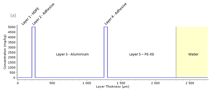
Fig. 49 – Initial spatial concentration profile C(x,t) of the migrant (maleic acid), essentially contained in the two adhesive layers.
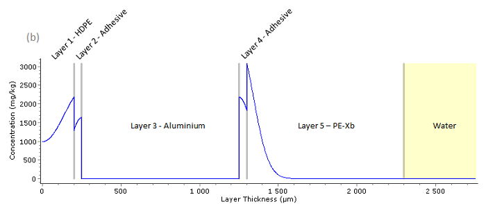
Fig. 50 – Spatial concentration profile C(x,t) of the migrant (maleic acid) after 10 days at 23°C
At 23°C the PE-Xb layer acts as a functional barrier and no migration of maleic acid from the pipe to drinking water is observed after 10 days. The migrant concentration profile C(x,t) in figure (b) clearly confirms that the maleic acid present in the adhesive layer penetrates only slightly through the PE-Xb layer. The same result, i.e. no migration of maleic acid from the pipe to drinking water is observed for the extended test cycle of 31 days.
The following figures shows the migration of maleic acid from the pipe to drinking water during 35 days at 60°C (test applied for the warm water: 1 + 3 x 1 + 3 + 3 x 1 days): the figure (a) presents the initial spatial concentration profile C(x,t) of the migrant (maleic acid), the figure (b) shows the spatial concentration of migrant C(x,t) in the pipe after 35 days, figure (c) presents the concentration of maleic acid C(t) in water as a function of time.
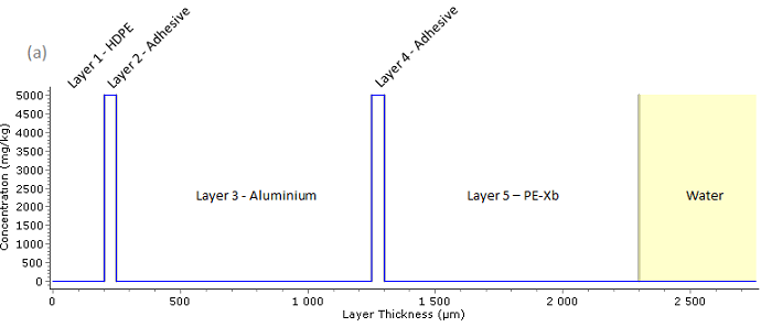
Fig. 51– Initial spatial concentration profile C(x,t) of the migrant (maleic acid), contained in the two adhesive layers
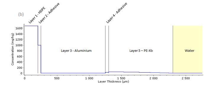
Fig. 52– Spatial concentration profile C(x,t) of the migrant (maleic acid) after 35 days at 60°C
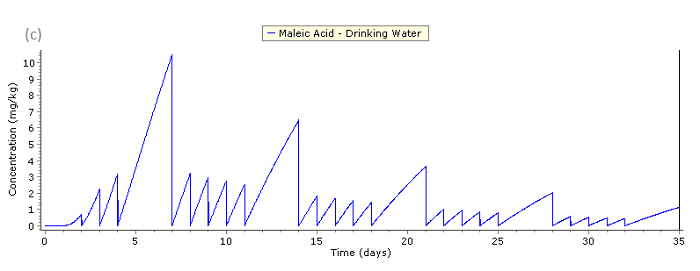
Fig. 53 – Concentration of the migrant (maleic acid) C(t) in water as a function of time
The estimated amount of maleic acid migration from the pipe to drinking water is 1.718 mg/l as presented in the above figure and in the table below.
The migration simulation was performed under “realistic” conditions, i.e. mean AP-value (polymer specific constant used to estimate the diffusion coefficients) of the distribution was used, therefore it can be expected that the estimated result is close to an experimental result obtained under the same testing conditions.
Set-off function
Introduction
During production and processing food contact materials and articles are stored often on the reel or in the stack where the inner food contact layer of the material or article comes into contact with the next outer layer. In such situation the transfer of migrants from the outer layer (such as e.g. printing ink) to the food contact layer (e.g. sealing layer) may occur. The set-off function is an in-built functionality which simulates migration in the reel or in the stack during storage when the material or article is brought into contact with food or food simulant and the specific migration is simulated according to the conditions of use or testing.
Example
Conical aluminum tubes with an inside placed protective coating containing the authorized migrants and a decorative printing placed outside containing ‘permitted’ migrants (based on risk assessment).
Set-off during storage
The conical tubes are stored in the stack prior to filling during which set-off, i.e. transfer of migrants from the decorative printing to the protective coating occurs as displayed in the picture :
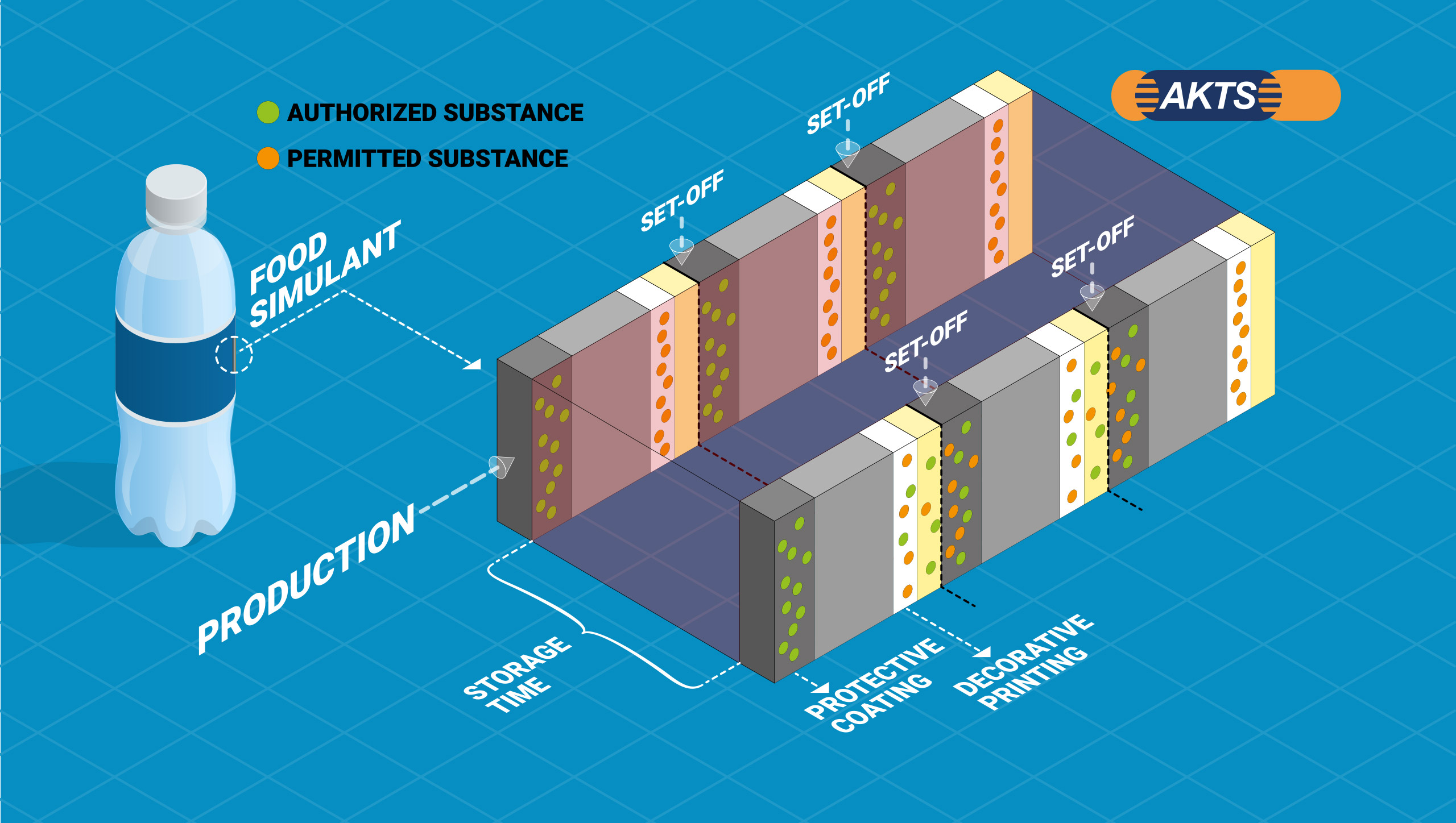
Fig. 54 – Conical tubes stored in the stack prior to filling.
Migration testing for compliance
‘Permitted’ substances may be identified in the layer of the protective coating due to set-off, despite the fact that direct migration from outside to inside through the material structure (in this example aluminum) is not possible.
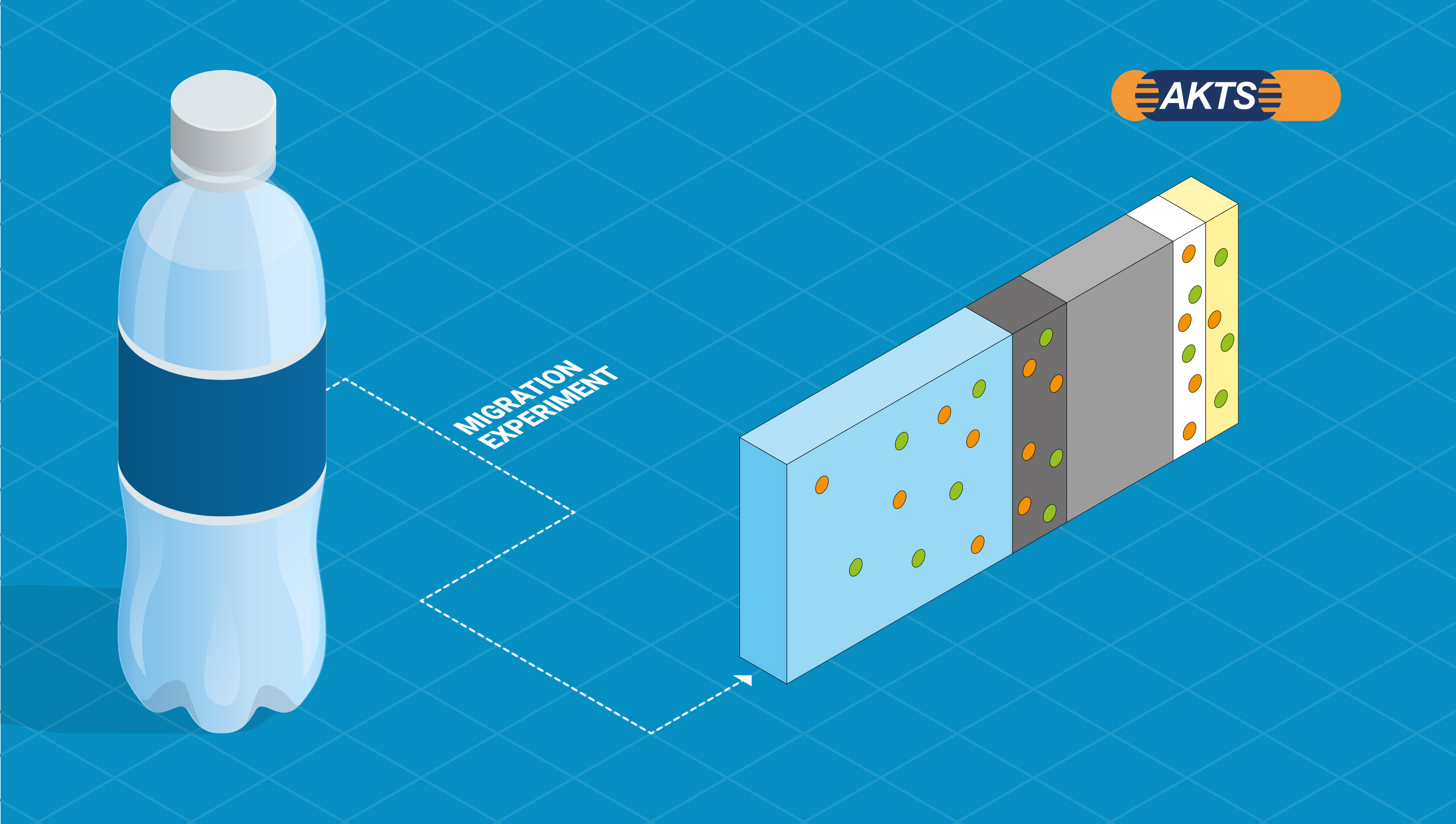
Fig. 55 – Migration testing for compliance.
- food contact layer contamination depending on sample history;
- detectable migration of authorized and ‘permitted’ substances (based on risk assessment);
- must comply with Article 3 of the Framework Regulation (EC) N°1935/2004
Summary
Set-off must be considered if food contact materials or articles are stored on the reel or in the stack before filling. The extent of set-off for individual migrants depends on their migration rates and relative solubility in the relevant layers (diffusion and partitioning) and is time and temperature dependent, i.e. depends on the material storage history.
The set-off function implemented in the SML 5 software simulates both the set-off process occurring in multilayer materials or articles and the migration process after filling. Hence the SML 6 software will support in evaluating specific migration issues, i.e. compliance assessment for authorized substances and/or risk assessment for “permitted” substances.
Calculation of Cmod in recycled PET
Summary
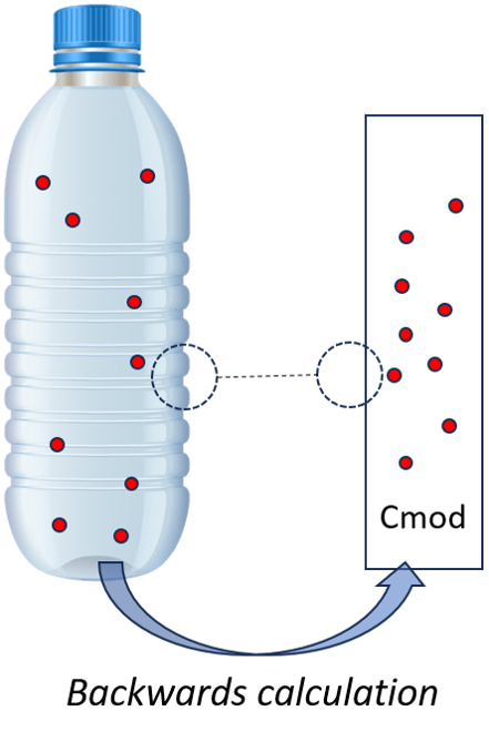
In the European Union, the safety evaluation of a PET recycling process is performed by comparing the residual concentration of each contaminant in recycled PET (Cres) to a modelled concentration (Cmod) in PET [1]. This Cmod is calculated using generally recognized conservative migration models and it corresponds to a migration which cannot give rise to an unsafe dietary exposure.

This application note describes how to apply the fitting model in AKTS-SML software to calculate Cmod for a contaminant used in a challenge test performed for the determination of the cleaning efficiency.
[1] EFSA Panel on on food contact materials, enzymes, flavourings and processing aids (CEF); Scientific Opinion on the criteria to be used for safety evaluation of a mechanical recycling process to produce recycled PET intended to be used for manufacture of materials and articles in contact with food. EFSA Journal 2011;9(7):2184. [25 pp.] doi:10.2903/j.efsa.2011.2184.
Evaluation principles
Migration criterion
In the safety evaluation, EFSA considers that a contaminant present in recycled PET should not give rise to a migration in food which could result in a dietary exposure higher than 0.025 µg/ kg bw/day.
Three exposure scenarios are considered. For the infants, the population group the most at risk, the exposure limit is respected if the concentration in water is lower or equal at 0.1 µg/ kg (modelling over-estimation factor of 5 included).
Cmod is the concentration in recycled PET that leads to a migration equal to 0.1 µg/kg food, using migration modelling.
Evaluation principles
Modelling parameters
For the Cmod calculation (infant scenario), EFSA requires the following parameters to be applied in the modelling:
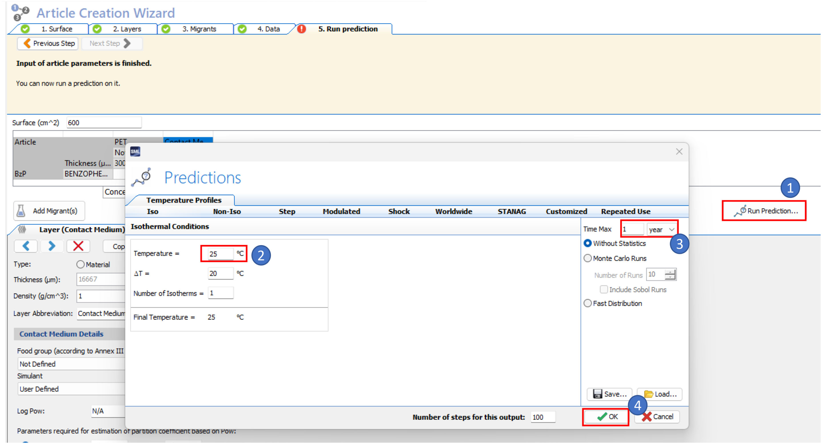
Contact time: 12 months
Contact temperature: 25°C
Thickness of PET package: 300 µm
Density of PET material: 1.375 g/cm3
Packaging geometry: EU-cube (V=1l, S=6dm2)
Diffusion coefficient, D: estimated with Piringer model (Ap’ = 3.1, Tau = 1577, worst case for T ≤ 70°C )
Partition coefficient, Kp/F 1.0 (good solubility)
Solving problem step by step
- Create the traditional “EU cube” package (volume of 1 l, surface of 600 cm2), one layer PET of 300 µm
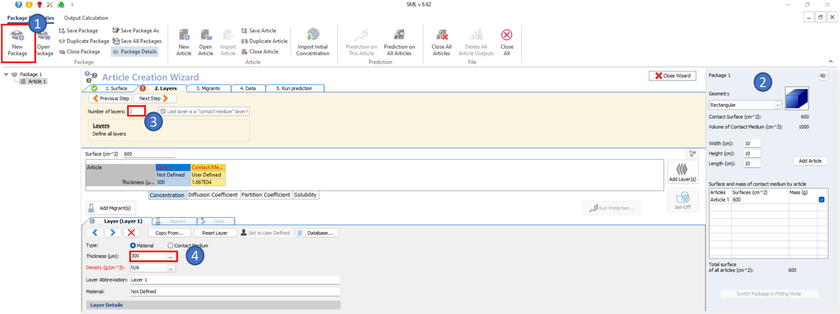
- Define the characteristics of the PET layer in the tab “set to User Defined” (alternatively, material type can be selected and assigned using the database)

- Select one migrant using the database (note: benzophenone is a common surrogate in challenge test of PET recycling process)
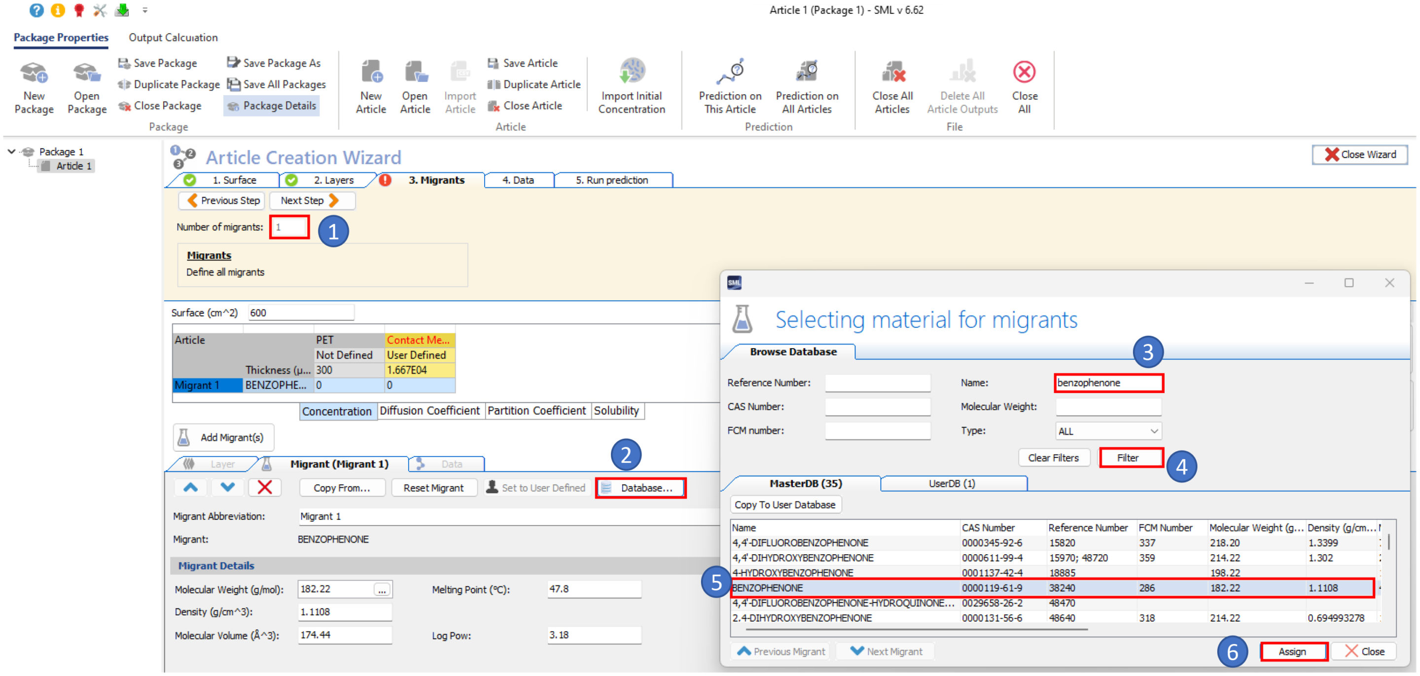
- Assign an initial concentration of benzophenone in the PET material

Note: the initial concentration of the contaminant is not important as it will be fitted backwards.
- Select the Piringer model for the estimation of the diffusion coefficient, then define the partition coefficient Kp/f equal to 1.0

- Enter the density of the contact medium (water)

- Run a prediction of the diffusion for the benzophenone
- Then import the migration criterion from a predefined file (migration infant scenario.txt)
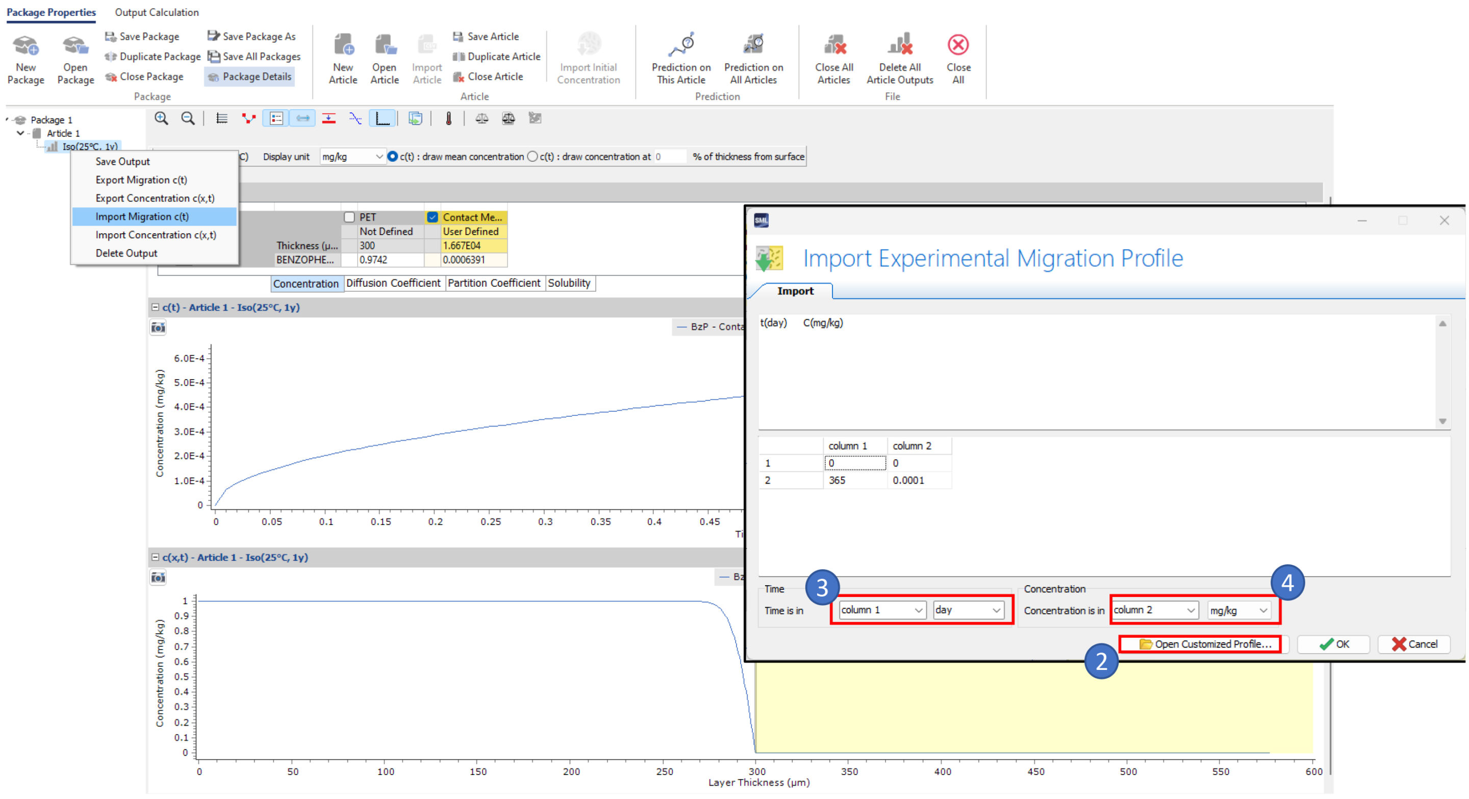
- Switch the package in fitting mode…
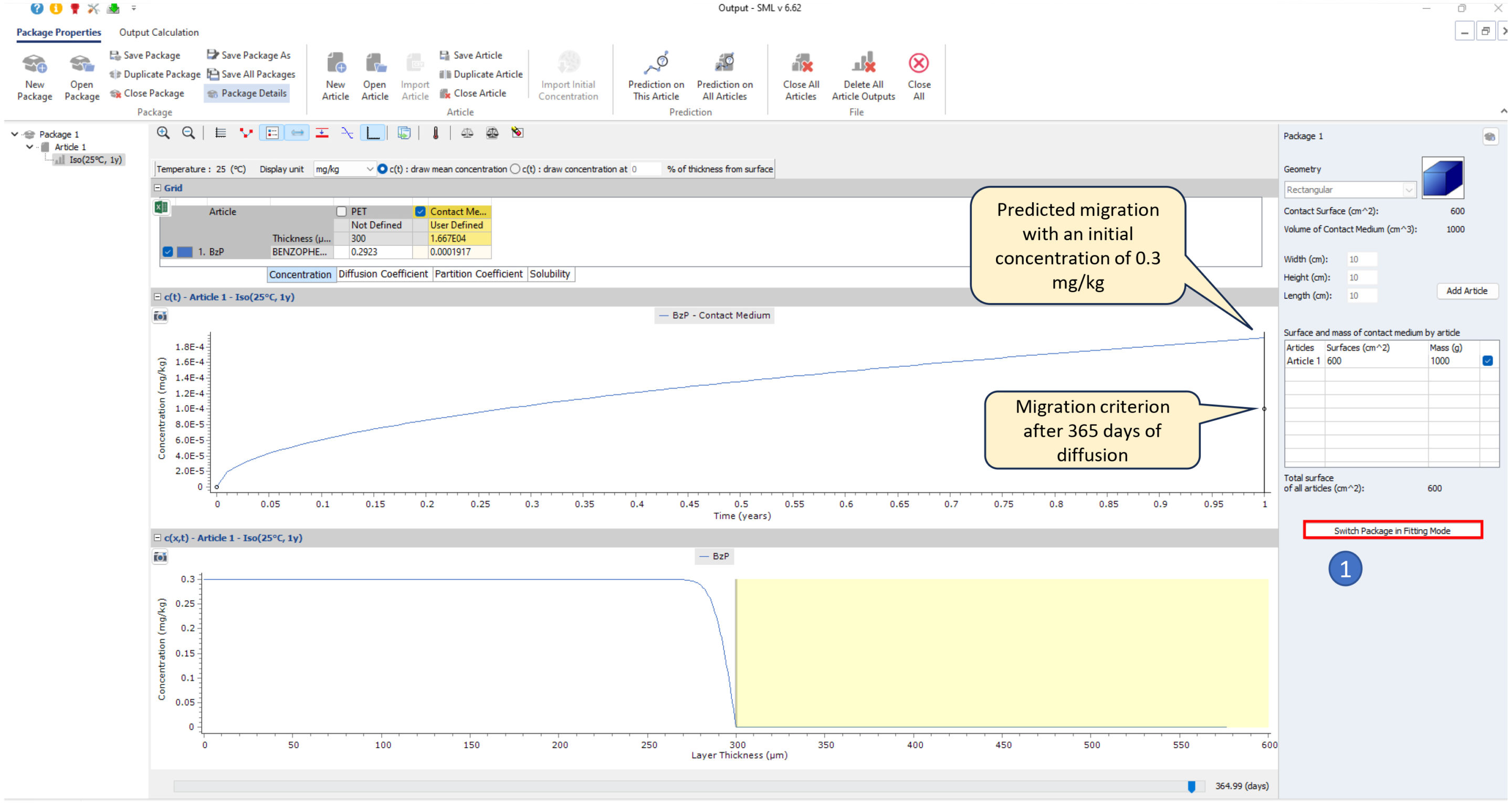
- …and chose to optimize the initial concentration in PET
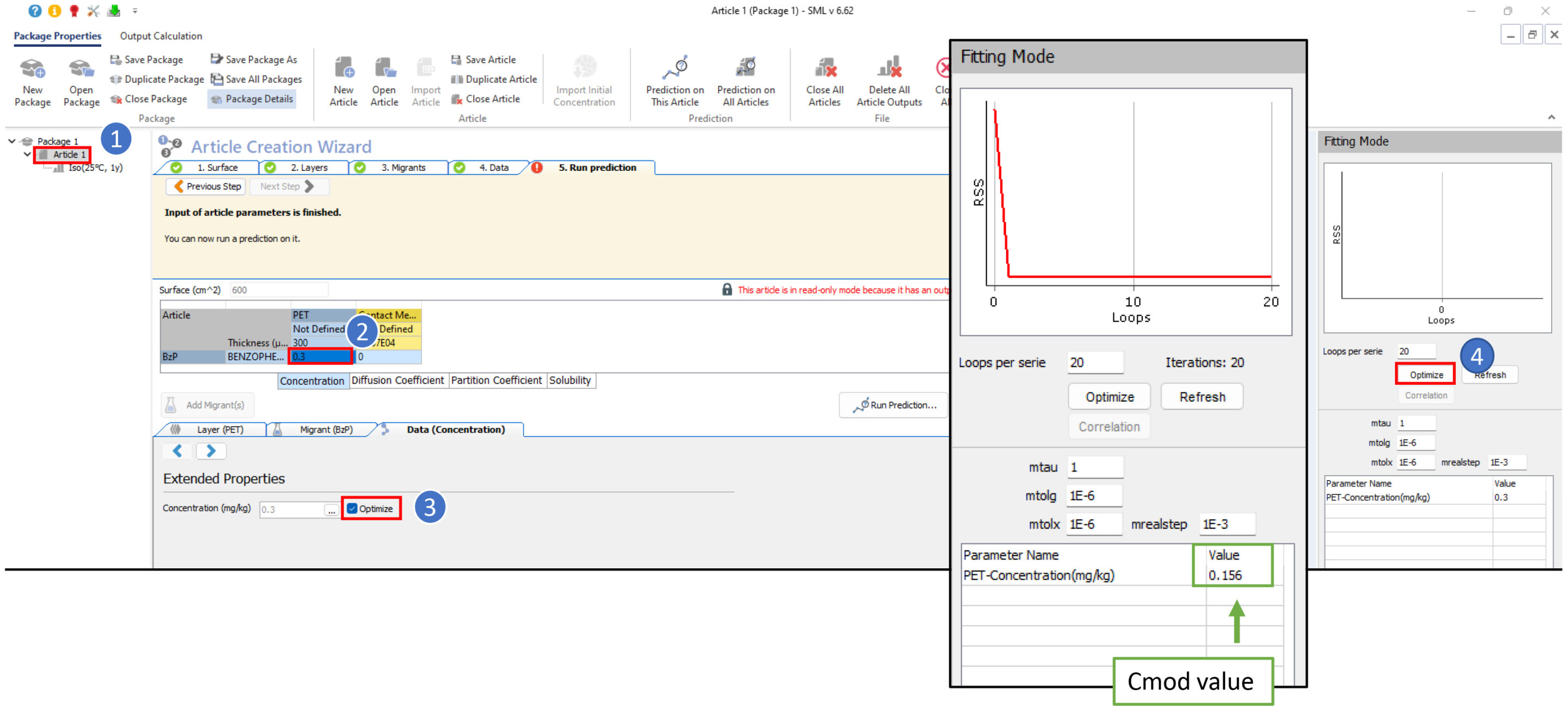
Note: if the difference between the migration criterion and the predicted migration is too large, the fitting module may have difficulty optimising the Cmod value. The value of the initial concentration must then be adapted.
Final remarks
This calculation can be adapted to fit different scenarios (i.e. EFSA scenarios for toddler or adult) or to calculate Cmod of other surrogates used in challenge test of PET recycling process: use the prepared package “Cmod_calculation” and enter the parameters of the desired migrant.
Also, the contact time or the temperature of the articles can be modified to evaluate packaging other than bottles.
Diffusion of photoinitiators into food simulant from real package
Summary
Flavoured milks, packed in a multilayer package are contaminated by different photoinitiators. The contamination occurs during the storage time of the printed material, by set-off, when the food contact layer stays in contact with the external layer.

The migration of photoinitiators into food simulant is measured to determine the real values diffusion coefficients.
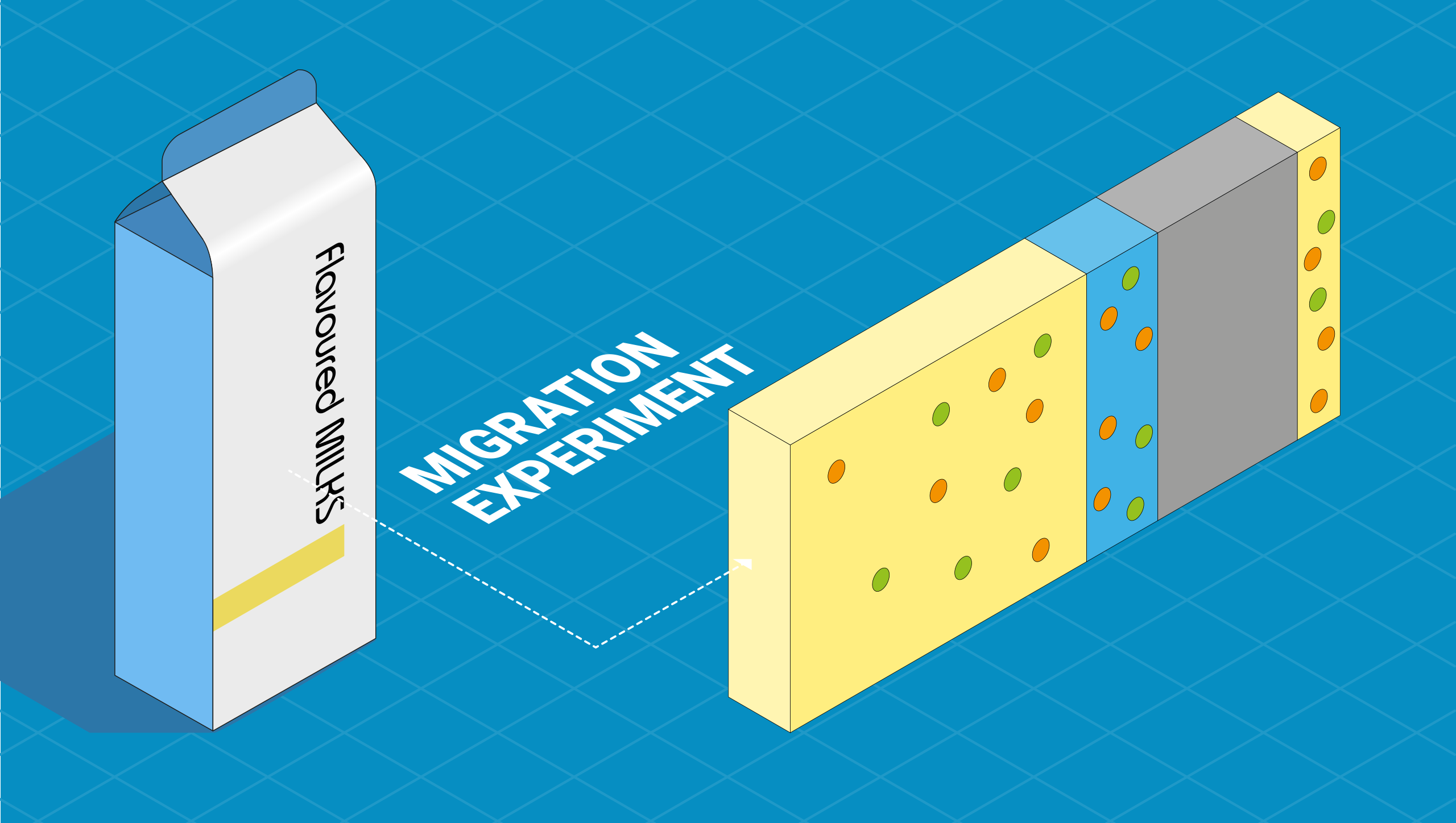
This application note shows how to extract the different diffusion coefficients of each photoinitiator from the experimental data and to how to find the initial concentration in the food layer with the fitting mode.
Experimental
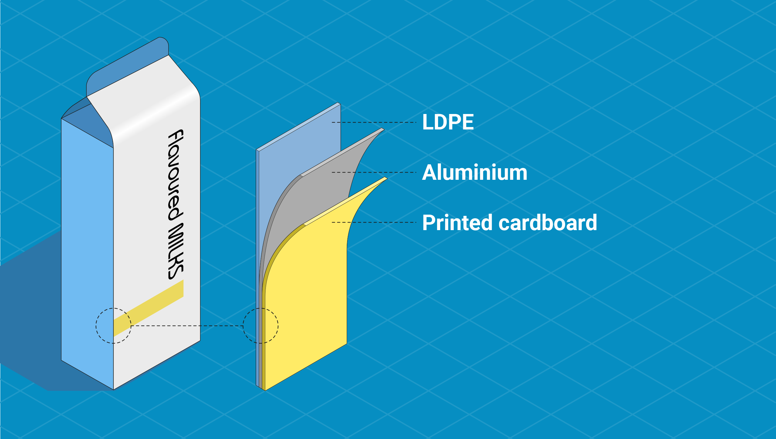
Material
The package is a multilayer cardboard/aluminium/LDPE with the cardboard surface printed (offset printing with UV-curing). The LDPE layer is 40 µm thick and is in contact with the food.
The three photoinitiators used to cure the ink are:
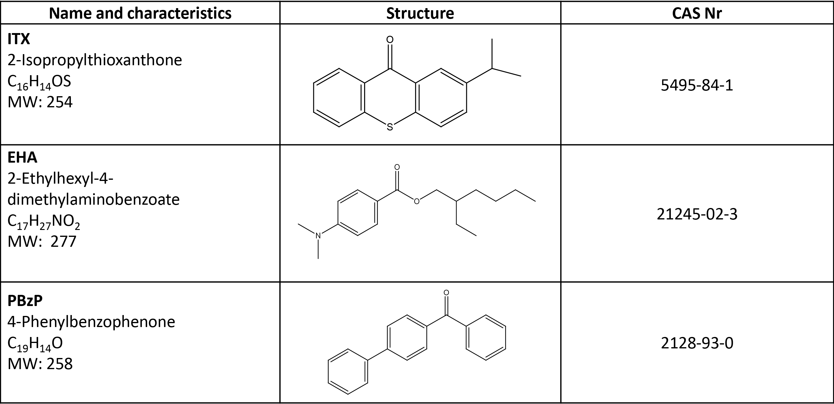
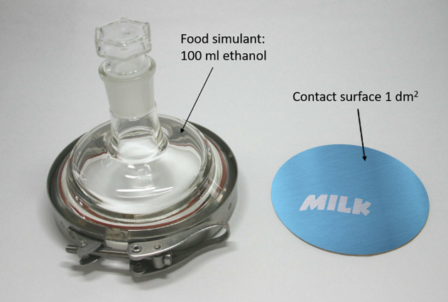
Experimental setup and conditions
The migration of photoinitiators from the LDPE layer into ethanol 95% (food simulant) is measured at 20°C. A one-side diffusion cell with a contact surface of 1dm2 and a volume of 100ml is used for the test. The initial concentration of photoinitiators in the LDPE, after set-off, is not measured and is unknown.
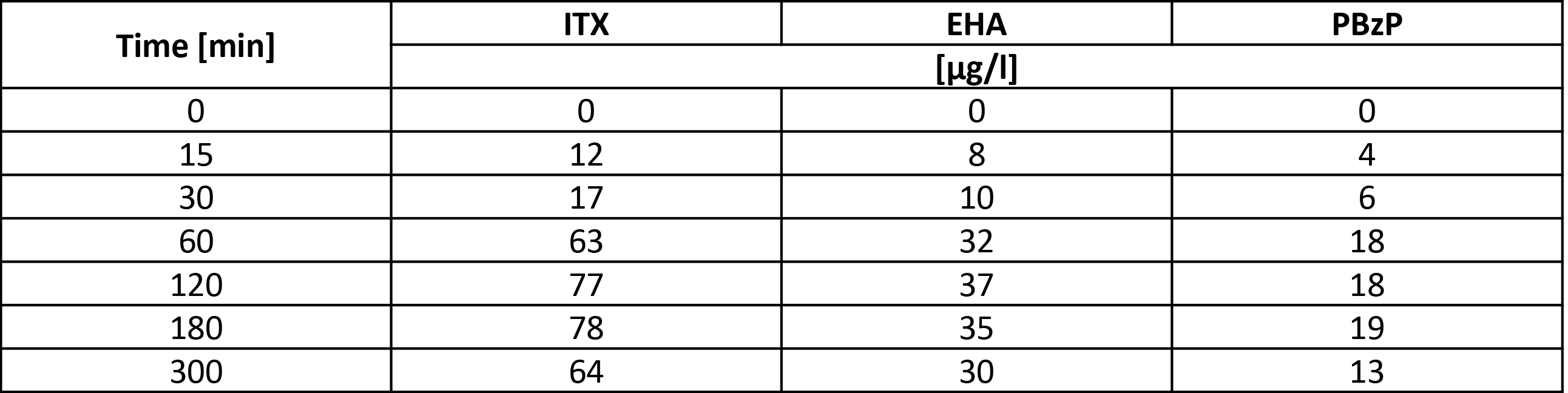
Measured data
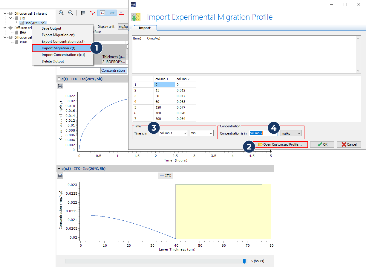
The concentration measured during the experiments are indicated in the table below.
Solving problem step by step
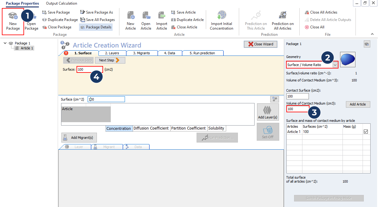
- Define the package corresponding to the experimental diffusion cell by using the surface/volume ratio geometry.
- Define the characteristics of the layers (only two are necessary, as the aluminium layer acts as a barrier layer). Material type can be selected using the database.
…repeat step 2 for the contact medium layer
- Add the migrants using the database The initial concentration of the photoinitiators was not assessed and is unknown. As the concentration in the ink layer is high (5%), the concentration in the LDPE can be high as well. Use a first estimate of 5 mg/kg (0.01% set-off).
…repeat step 3 for all migrants

- Estimate the diffusion coefficients of the photoinitiator using the Piringer model.
- Define the partition coefficients between the LDPE layer and the food simulant as 1 (worst case).
- Duplicate this package twice to get one package per photoinitiator. Rename each article for one photoinitiator and delete the other two migrants.

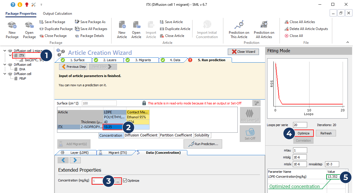
- Run a prediction for the first photoinitiator (ITX)
- Then import the experimental data from a predefined file (migration ITX_20C.txt)
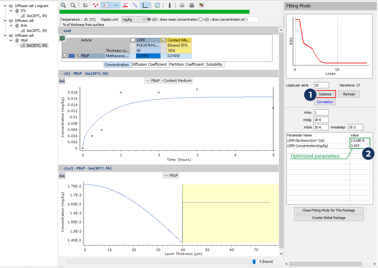
- Switch the package in fitting mode…
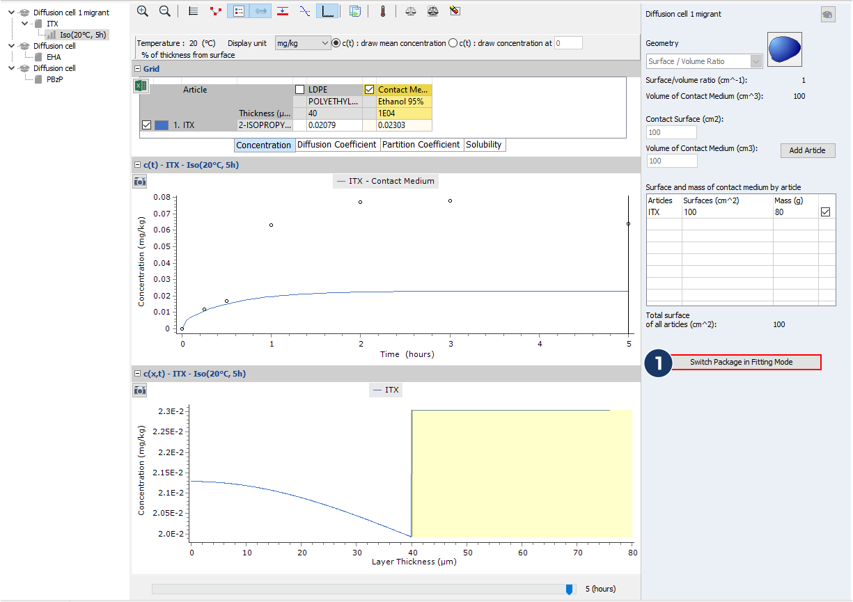
- …and optimize the initial concentration
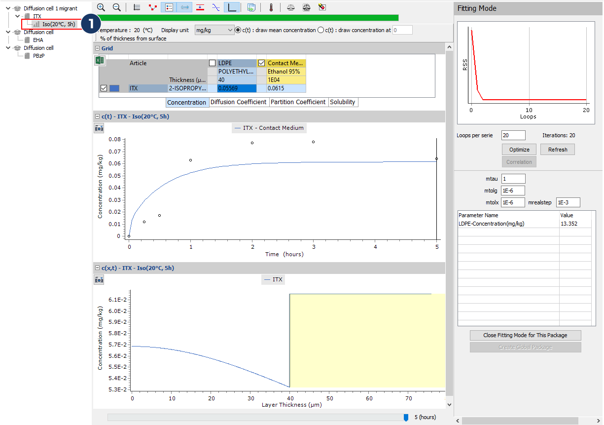
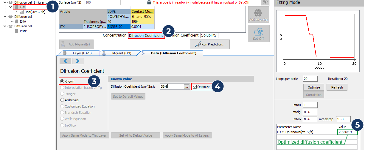
- Unselect the optimisation of the concentration and optimize the diffusion coefficient
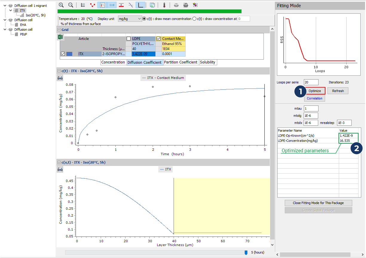
- Select to optimise both the concentration and the diffusion together and launch the fitting process again.
- Repeat this process from step 7 on the two other packages and optimize the initial concentration and the diffusion coefficient for the two other photoinitiators
Expected results

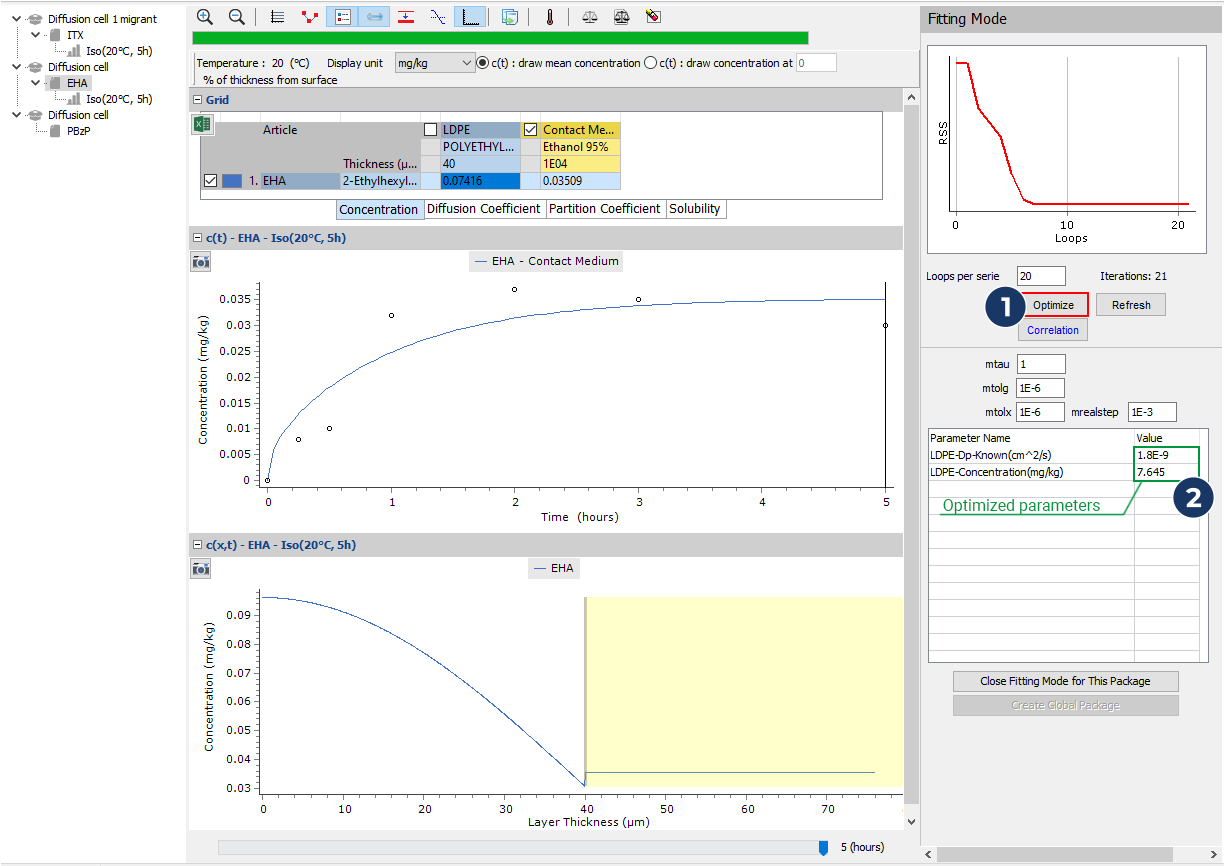
- Results for EHA
- Results for PBzP