Detailed description
THERMAL SAFETY Software (TS)
The THERMAL SAFETY Software (TS) is based on different approach than those applied in the Thermokinetics (TK) and Thermokinetics Sparse Data (TKsd) Software. For the prediction of the thermal behavior of the materials in kg and ton scale not only kinetic analysis but also the heat balance in the system is considered. Thermal Safety Software allows the determination the safety parameters of the process occurring in adiabatic (Time to Maximum Rate, TMRad) – or semi-adiabatic conditions (Self Accelerating Decomposition Temperature, SADT).
Introduction
The precise prediction of reaction progresses in adiabatic conditions is necessary for the safety analysis of many technological processes. Calculations of an adiabatic temperature-time curve for the reaction progress can also be used to determine the decrease of the thermal stability of materials during storage at temperatures near the threshold temperature. Due to insufficient thermal convection and limited thermal conductivity, a progressive temperature increase in the sample can easily take place, resulting in a thermal runaway.
Several methods have been presented for predicting reaction progress of exothermic reactions under heat accumulation conditions [1, 8-17, 23-44]. Because of decomposition reactions usually have a multi-step nature, the accurate determination of the kinetics is a key prerequisite for correct describing the progress of the reaction. The use of simplified kinetic models for the assessment of runaway reactions can, on one hand, lead to economic drawbacks, since they result in exaggerated safety margins. On another hand, it can cause dangerous situations when the heat accumulation is underestimated. For strongly exothermic reactions occurring adiabatically, incorrect kinetic description of the process is usually the main source of prediction errors.
Basic Concept of the Thermal Safety Analysis
- advanced determination of the reaction kinetics, which properly describes the complicated, multistage course of the decomposition.
- The evaluation of the effect of heat balance, as the sample mass is increased by a few order of magnitude compared to the thermoanalytical experiments.
Because decomposition reactions usually have a multi-step nature, the isoconversional analysis enables a more accurate determination of the kinetic characteristics compared to simplified kinetic assumptions like ‘let’s assume that the reaction is zero-th (or 1-st) order etc.’
The application of the DSC data for the simulation of the adiabatic measurements seems to be, at the first glance, not obvious. However, the closer look on the differences and similarities of the processes occurring under different conditions of the heat exchange allows to understand that the adiabatic properties such as self-heating rate or time to maximum rate can be correctly determined from the DSC results obtained or isothermally, or better, at different heating rates. The main difference between DSC run and fully adiabatic process lays in the conditions of the heat exchange. Due to the fact that in the thermoanalytical experiments the heat evolved during reaction is fully exchanged with the environment, the heating rates under which the experiments are carried out can be arbitrarily chosen. In turn, after determination of the kinetic parameters from the results of few experiments done with different heating rates, one can predict the reaction rate under any temperature ramp.
Due to the totally different rate of heat exchange in adiabatic conditions the heating rate of the process (called now self-heating rate) cannot be controlled anymore, being dependent now on the kinetics, adiabatic temperature rise and φ-factor. Experimental data collected during investigation of exothermic reactions in adiabatic conditions must be corrected for the effect of sample container heat capacity. This correction factor is called the phi factor or thermal inertia (Townsend and Tou [24]). The heat capacity of the container (test cell) serves to lower the measured temperature of the reaction and increase the time to maximum rate. The thermal inertia is defined as φ= (heat capacity of the sample + heat capacity of the vessel)/ heat capacity of the sample. The phi-factor approaches the value of 1 for large vessels or at genuine adiabatic conditions.
The scheme of the general idea of the application of the DSC data for the simulation of the adiabatic measurements is presented in the next figure.
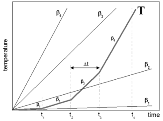
Fig. 1 – Scheme of the representation of the adiabatic temperature rise by four sequences of the time periods Δt in which the heating rates are constant and amount to β1, β2, β3 and β4, respectively.
Let us assume that the temperature increase under adiabatic conditions in the coordinates time temperature can be presented schematically as in Fig. 1 in the form of four sequences of the short periods of time Δt in which the heating rate is constant. In time periods 0-t1, t1-t2, t2-t3 and, finally, t3-t4 the heating rates are β1, β2, β3 and β4, respectively. Using the commonly applied kinetic analysis as e.g. this one which is implemented in AKTS-Thermokinetic (TK) software one can easily predict the reaction rate under any heating rate β value. During the temperature change schematically presented in Fig. 1, the reaction course can therefore be calculated as a sequence of processes occurring at known heating rates β1-β4. Using the infinitesimal Δt values for the description of the self-heating rate one can predict the reaction course under the adiabatic temperature change. The process occurring under adiabatic temperature rise is expressed as a succession of an infinite numbers of processes occurring at constant heating rates which can now be easily calculated by conventional kinetic methods.
Heat transfer mechanisms
The heat is the form of energy that can be transferred from one system to another system as a result of temperature difference.
Heat can be transferred in three basic modes:
- Conduction
- Convection
- Radiation
Conduction
Conduction is the transfer of energy from the more energetic particles of a substance to the adjacent less energetic ones as a result of interactions between the particles. Conduction can take place in solids, liquids, or gases. In gases and liquids conduction is due to the collisions and diffusion of the molecules during their random motion. In solids, conduction is due to the combination of vibrations of the molecules in a lattice and the energy transport by free electrons.
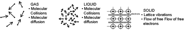
Fig. 2 – Heat transfer by conduction in solids, liquids or gases.
The range of thermal conductivities λ is enormous. As shown in Fig. 2, λ varies at room temperature by a factor of about 104 between gases (poor heat conductor or insulator) and metals (good heat conductor).
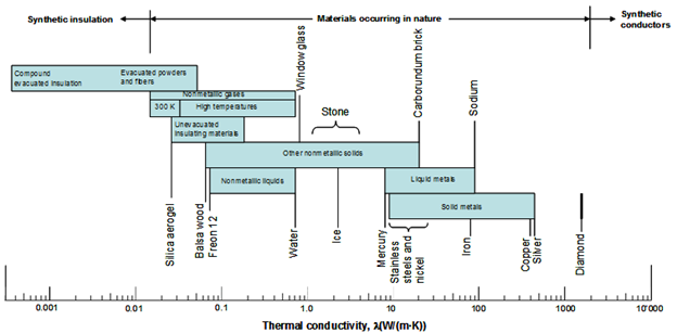
Fig. 3 – Thermal conductivities of materials. Pure crystals and metals have the highest thermal conductivities, and gases and insulating materials the lowest.
Convection
Convection is the mode of energy transfer between a solid surface and the adjacent liquid or gas that is in motion. Convection is commonly classified into three sub-modes:
- Forced convection
- Natural (or free) convection
Radiation
Radiation is the energy emitted by matter in the form of electromagnetic waves (or photons) as a result of the changes in the electronic configurations of the atoms or molecules. Heat transfer by radiation does not require the presence of an intervening medium. Radiation is emitted by bodies because of their temperature. All bodies at a temperature above absolute zero emit thermal radiation.
The kinetic based approach for the determination of the Time to Maximum Rate under adiabatic conditions (TMRad)
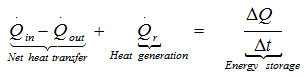
Heat balance of the system requires the evaluation of the amount and the rate of the heat generated during chemical exothermic reaction and the amount and rate of the heat exchanged with the environment. The rate of the heat generation can be evaluated by the kinetic analysis of the investigated reaction. The knowledge of the kinetics parameters is a very important prerequisite of the correct heat balance which allows the precise prediction of the thermal behavior of the semi-and fully adiabatic systems. The solution of the general heat balance equation.
allows the construction of thermal stability diagram, in which the Time to Maximum Rate under adiabatic conditions (TMRad) can be predicted for any arbitrarily chosen starting temperature.
Batch reactor in case of cooling failure
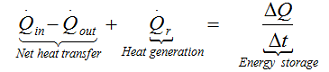
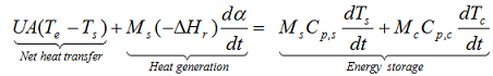
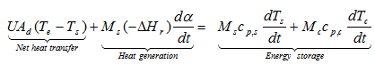
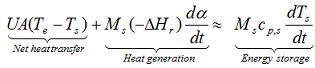
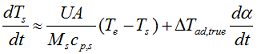
The energy balance of an exothermic reaction taking place in a batch reactor can be expressed as
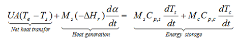
with M: mass, Cp: specific heat, T: temperature, U: overall heat transfer coefficient, A: contact surface between the sample and the container, ΔHr: heat of reaction, indices c, s and e: are used for container, sample and environment, respectively. In case of cooling failure the overall heat transfer coefficient U=0 for achieving the adiabatic conditions. In a fully adiabatic conditions all the heat released during reaction increases the temperature of the sample and the container. If there is thermal equilibrium within the reacting medium and the wall of the reactor.
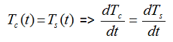
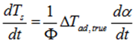
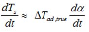
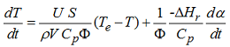
then the whole system will have the same temperature rise rate and we can simplify the above equation to:
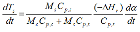
that can be rewritten as
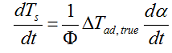
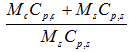
with:
the adiabatic temperature rise:
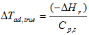
the phi factor φ =
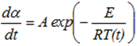
the reaction rate
![]()
For batch reactor with large sizes (>1m3), it can be assumed that Ms >>Mc (jacket) so that we obtain
![]()
![]()
Applying the isoconversional analysis we have:
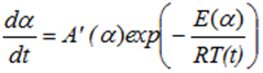 with
with ![]()
where E(α)em> and A(α)em> represent the values of the activation energy E and pre-exponential factor A at the specific conversion extent α.
Note, that in case of simplified zero order kinetic assumption we have:
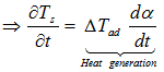
Presented above equations are used in kinetic based approach for predicting the reaction progress α(t) and rate dα/dt as well as the development of the temperatures Ts (t) and dTs /dt and adiabatic induction times at any selected starting temperatures.
Adiabatic calorimeter
There are several issues that need to be taken into consideration for the examination of adiabatic conditions or reconstructing an Accelerating Rate Calorimeter experiment when applying the kinetic based approach. The energy balance in case of an adiabatic calorimeter can be expressed as before
Because the presence of a temperature difference leads to heat transfer, an adiabatic calorimeter constantly attempts to achieve the equilibrium state by keeping Te = Ts. As a consequence there is no driving force for a heat transfer and the chemical reactions run adiabatically. We obtain as before
![]()
However, one has to take into account the thermal inertia (φ-factor) to consider the effect of the vessel’s inertia i.e. the reaction heat that is transferred in part into heating reactor walls. The value of φ-factor has to be considered during the simulation of an ARC experiment. The φ-factor influences :
(i) The ![]() because it comes from above description that
because it comes from above description that
(ii) The TMRad depending on the type of decomposition kinetics.
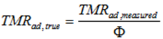
Usually, the approximated equation correcting the time for the reaction under adiabatic conditions is expressed as
Dewar
In Dewar tests the energy balance can be handled just like exothermic reaction in the adiabatic calorimeter or in batch reactor in case of cooling failure.
The net heat rate through a typical for Dewar three-layered wall (glass-vacuum-glass) of thicknesses L1, L2 and L3 with convection on both sides is presented in the figure:
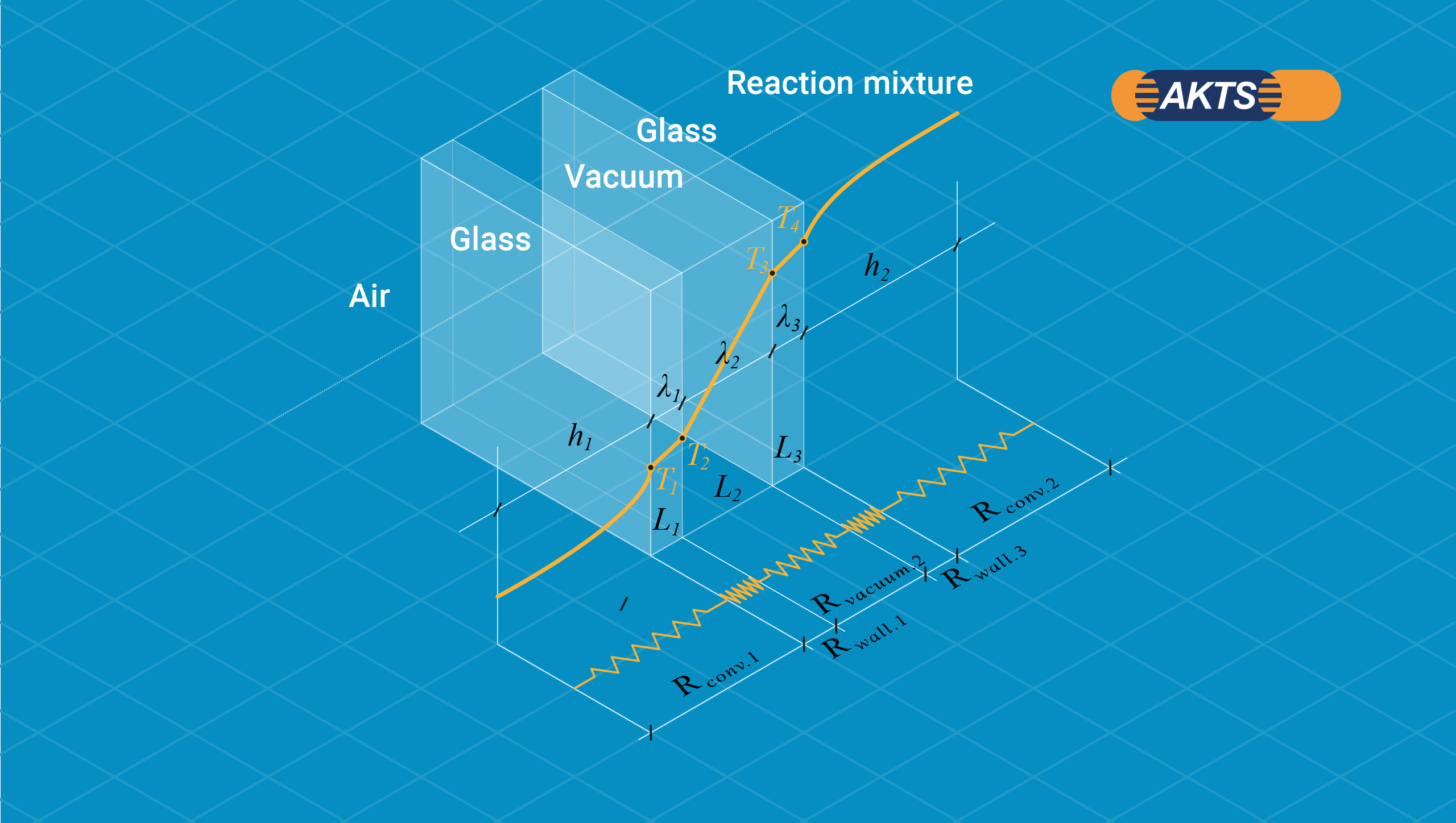
Fig. 4 – Schematic description of a heat balance in a Dewar: the net heat rate through a three-layered wall (glass-vacuum-glass) of thicknesses L1, L2 and L3 with convection on both sides.
Picture to be redone
The heat transfer between air and the wall at the outer surface occurs by convection whereas through the three-layered wall it occurs by conduction. If the reaction mixture is a liquid, the heat transfer between the reactants and the wall at the inner surface proceeds by convection. Rate of heat convection into the wall, rate of heat conduction through the wall and rate of heat convection from the wall can be expressed as:
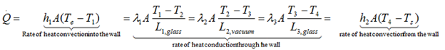
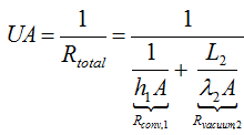
According to Newton’s law of cooling one can express the heat transfer through a medium UA(Te-Ts) using the thermal resistance concept:
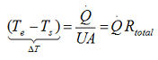
where
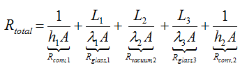
As h1<< h2, λ1<<λ2 and λ3<<λ2
h1<< h2, λ1<<λ2 and λ3<<λ2 (because λvacuum<<λglass), it can be assumed that
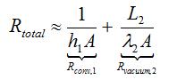
In addition, Ms>>Mc(glass) so that after insertion into the energy balance
and simplification we can write
![]()
Note that
If the total resistance Rtotal is very large it can be assumed that U → 0 and we obtain
which leads basically to the same expression as before for exothermic reaction in the adiabatic calorimeter or batch reactor in case of cooling failure
Time to Maximum rate under adiabatic conditions (TMRad)/ Thermal Safety Diagram
Construction of a thermal safety diagram: runaway time as a function of process temperature under adiabatic conditions (TMRad = ƒ(T))
The decomposition of the examined substance is exothermic with the heat of reaction ΔHr = -554.8 ±17.4 J/g. Assuming a heat capacity Cp = 1.5 J/(g·K), one can calculate the reaction progress due to self-heating for any ΔTad = (-ΔHr)/Cp/Φ.
The adiabatic induction time is defined as the time which is needed for self-heating from the initial temperature to the time of maximum rate (TMRad) under adiabatic conditions. Depending on the decomposition kinetics and ΔTad, the choice of the initial temperature strongly influences the time to runaway and the rate of the temperature evolution under adiabatic conditions. Figure 5.5 presents the dependence of the adiabatic induction time TMRad on the initial temperature.
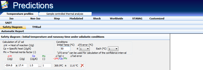
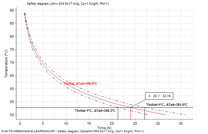
Fig. 5 – Thermal safety diagram: Influence of the initial temperature on corresponding adiabatic induction time TMRad for following conditions : ΔHr = -554.8±17.4 J/g and ΔTad=(-ΔHr)/Cp/Φ=369.9±11.6°C for Φ = 1 and Cp = 1.5 J/g/°C.
ΔHr = -554.8±17.4 J/g, Cp = 1.5 J/g/K, ΔTad=(-ΔHr)/Cp= 369.9±11.6°C |
|||
|---|---|---|---|
Temperature (°C) | Time (h) | Time (h) | Time (h) |
| 89 | 0.95 | 0.87 | 1.05 |
| 88 | 1.03 | 0.94 | 1.14 |
| 87 | 1.12 | 1.02 | 1.24 |
| 86 | 1.21 | 1.1 | 1.34 |
| 85 | 1.32 | 1.19 | 1.46 |
| 84 | 1.43 | 1.29 | 1.58 |
| 83 | 1.55 | 1.4 | 1.72 |
| 82 | 1.69 | 1.52 | 1.87 |
| 81 | 1.83 | 1.66 | 2.03 |
| 80 | 1.99 | 1.8 | 2.21 |
| 79 | 2.17 | 1.96 | 2.4 |
| 78 | 2.36 | 2.13 | 2.62 |
| 77 | 2.57 | 2.32 | 2.85 |
| 76 | 2.8 | 2.52 | 3.11 |
| 75 | 3.05 | 2.75 | 3.39 |
| 74 | 3.33 | 3 | 3.71 |
| 73 | 3.63 | 3.27 | 4.05 |
| 72 | 3.97 | 3.57 | 4.42 |
| 71 | 4.34 | 3.89 | 4.83 |
| 70 | 4.74 | 4.25 | 5.29 |
| 69 | 5.18 | 4.65 | 5.79 |
| 68 | 5.67 | 5.08 | 6.34 |
| 67 | 6.21 | 5.56 | 6.94 |
| 66 | 6.8 | 6.09 | 7.61 |
| 65 | 7.46 | 6.67 | 8.35 |
| (*)64 | (*)8.18 | (*)7.31 | 9.16 |
(*) Means that if Φ=1 and Cp=1.5 J/g/°C the determined TMRad is about 8 hours (8.18 h) for an initial temperature of about 64°C (for that temperature a more conservative value for TMRad is about 7.31 h) |
|||
| 63 | 8.97 | 8.02 | 10.06 |
| 62 | 9.85 | 8.8 | 11.05 |
| 61 | 10.83 | 9.66 | 12.15 |
| 60 | 11.9 | 10.61 | 13.37 |
| 59 | 13.09 | 11.66 | 14.72 |
| 58 | 14.4 | 12.82 | 16.21 |
| 57 | 15.86 | 14.11 | 17.86 |
| 56 | 17.48 | 15.53 | 19.7 |
| 55 | 19.27 | 17.11 | 21.73 |
| 54 | 21.26 | 18.87 | 23.99 |
| (**)53 | (**)23.47 | (**)20.81 | 26.51 |
(**) Means that if Φ=1 and Cp=1.5 J/g/°C the determined TMRad is about 24 hours (23.47 h) for an initial temperature of about 53°C (for that temperature a more conservative value for TMRad is about 20.81 h) |
|||
| 52 | 25.92 | 22.97 | 29.3 |
| 51 | 28.65 | 25.37 | 32.42 |
| 50 | 31.69 | 28.03 | 35.88 |
Table 1 – Thermal safety table: Dependence of TMRad on initial temperatures under adiabatic heat accumulation conditions.
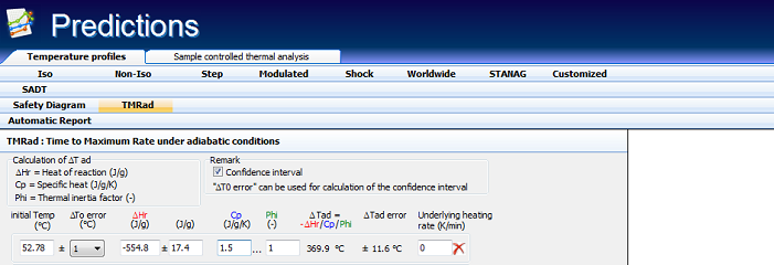
Fig. 6 – The simulation of T-time relationships under adiabatic conditions for an initial temperature of about 52.8°C leading to TMRad of 24 h.
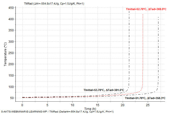
Fig. 7 – Adiabatic runaway curves for the reaction with ΔHr = -554.8±17.4 J/g and Cp = 1.5 J/g/K showing the confidence interval for the prediction: Tinitial =52.78±1°C. ΔTad=(-ΔHr)/Cp/Φ=369.9±11.6°C for Φ =1.
Note that isothermal conditions can be numerically retrieved by setting an exceptionally large value of φ to make the adiabatic temperature rise ΔTad insignificant. If the φ is very high all heat released in the reaction is dissipated to the surrounding. As a consequence, the sample temperature remains constant i.e. isothermal :
![]()
for very large values of φ we have
![]() and
and ![]()
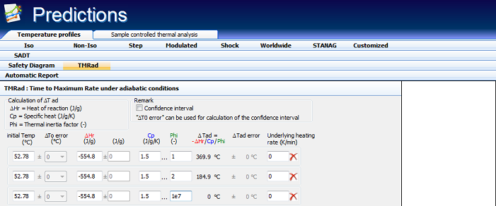
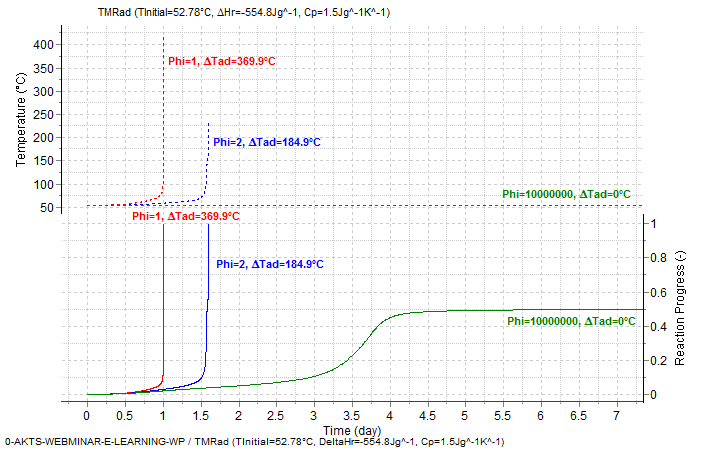
Fig. 8 – Comparison between the reaction progress and reaction rate under isothermal conditions (T=52.78°C, Φ = 1E10) and the adiabatic runaway curve with an initial temperature of 52.78°C with Φ = 2 and 1 (for Φ =1 TMRad amounts to 24h), respectively. ΔHr = -554.8±17.4 J/g and Cp = 1.5 J/g/°C.
The self-heat rate curves under adiabatic conditions are presented in Fig. 9 Self heat rate of 0.02 K/min (with Φ = 1), which corresponds to the typical detection limit of adiabatic calorimeters, is reached after about 17 hours, it means 7 hours before TMRad of 24 h for an initial process temperature of 52.78°C. At the time when the reaction rate reached the detection limit of typical adiabatic calorimeter the reaction progress amounts already to about 0.022 (about 2.2%) (Fig. 9).
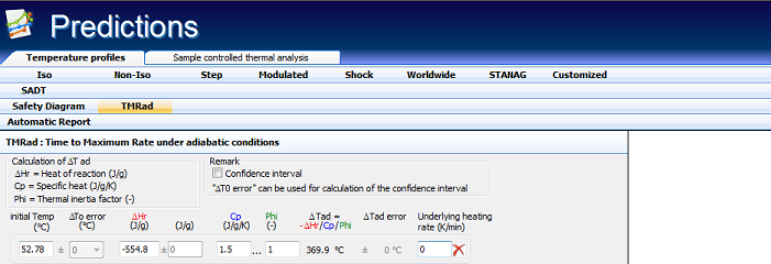
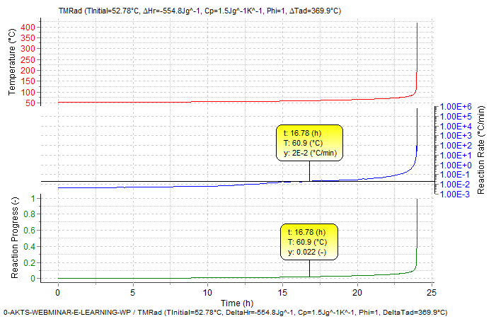
Fig. 9 – Adiabatic runaway curve with TMRad = 24h with corresponding reaction progress and self heating rate curve as function of time (ΔHr = -554.8±17.4 J/g and ΔTad=(-ΔHr)/Cp/Φ=369.9±11.6°C for Φ = 1 and Cp = 1.5 J/g/K).
Similar calculations can be performed for different phi-factors (see figures 10.) for an initial temperature of about 52.78°C.
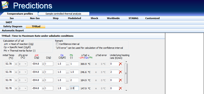
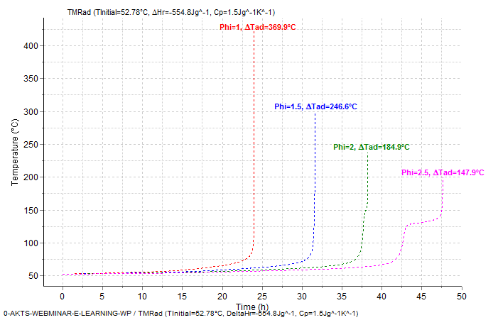
Fig. 10 – Thermal behavior of examined material under adiabatic conditions for different Φ factors. Adiabatic runaway curves (top) and self heat rate curves (bottom)
|
Φ |
ΔTad /K |
|---|---|
|
1 |
369.9 |
|
1.5 |
246.6 |
|
2 |
184.9 |
|
2.5. |
147.9 |
Table 2 – Influence of the Φ factor on the ΔTad at following conditions Tinitial =18.04°C, ΔHr = -554.8±17.4 J/g and Cp = 1.5 J/g/K
Self Accelerating decomposition temperature (SADT)
Introduction
Some chemicals have the potential to cause fires or explosions, and, as hazardous materials, are handled with appropriate care to minimize accidents. This category of hazardous materials includes a group of chemical substances called reactive or self-reactive chemicals which may initiate exothermic decomposition by themselves. The commonly applied thermal hazard indicator which estimates the hazard probability, especially for packaged materials during transport, and/or storage, is Self Accelerating Decomposition Temperature (SADT). The determination of SADT is based on the monitoring of the temperature of the sample with the mass m, volume V, surface area S, density (or bulk density) ρ, and specific heat capacity Cp, with a uniform initial temperature T0 and packed into a vessel of arbitrary shape. At time t0, the surrounding temperature of the investigated material is increased to Te which initiates the heat transfer between the packaged material and its surroundings, characterized by a heat transfer coefficient h. The SADT, as defined by the United Nations SADT test H.1 [41], is the lowest ambient temperature at which the centre of the material within the package heats to a temperature 6°C higher than the environmental temperature Te after seven days or less. This period is measured from the time when the temperature in the center of the packaging reaches 2°C below the ambient temperature. The determination of SADT according to UN test H.1 [41] is based on the results of series of large-scale experiments performed with the packaging in an oven at constant temperatures. Each test, performed at a new temperature, (according to the UN recommendations, the step of the oven temperature variations amounts to 5°C) requires a new large-scale packaging. This procedure, despite its reliability, is rarely used, because it is rather expensive, material- and time-consuming and, in certain cases, quite dangerous due to thermal safety and toxicity reasons. Another limitation is related to the relatively common situation when only a small amount of the investigated material is available at the early stages of a project. Taking into account all the issues presented above, it seems fully understandable that there is an important need of other reliable, faster, safer and cheaper test methods requiring smaller amounts of reactive materials and applicable at the laboratory scale (mg or g).
Due to the fact that significant amount of heat is evolved during the decomposition of self-reactive chemicals their thermal properties are frequently investigated in laboratory at mg- or g-scales under non-isothermal or isothermal conditions using Differential Scanning Calorimetry (DSC) or, more sensitive, Heat Flow Calorimetry (HFC). The elaboration of the heat flow data monitored by these both techniques allows determination of the kinetic parameters of the decomposition process which describe the rate of the heat generation in the conditions of the ideal heat exchange with the surroundings. However, during the scale-up not only kinetics but also the issue of the heat balance has to be considered as well. In kg-scale, due to increasing sample mass, the conditions of the heat exchange with the environment significantly change what, in turn, may considerably increase the reaction rate and the spatial evolution of the sample temperature which depends on:
- The kinetic and thermodynamic parameters of the reaction (activation energy, pre-exponential factor, reaction kinetic model, reaction heat)
- The physical parameters of the material (liquid or solid state, heat capacity, thermal conductivity, density), and
- The user-controlled parameters of the experiment (such as sample size, heating rate or temperature, type of packaging, rate of heat exchange with the surroundings, gas atmosphere, etc.)
Thus, once the kinetic parameters of the reaction are known, the temperature profiles for chosen sample size can be accurately estimated for any desired, user-controlled parameters by adequately applying the corresponding physical and thermodynamic parameters. Therefore, one can conceive the kinetic-based approach as a reasonable and possible support or even an alternative to the large-scale UN test H.1.
The important aspects of the kinetic workflow, i.e. the sequence of all the processes through which a kinetic analysis passes from initiation to completion, and the recommendations for proper collection of experimental data, have already been discussed in the last three ICTAC Kinetic Projects [2-7]. However, if intended for scale-up, the computational aspects of the kinetic analysis should be extended by additional recommendations about the collection of experimental data, thermodynamic and physical parameters, and the determination of the user-controlled parameters that adequately allow the accurate determination of the heat balance. Moreover, it is necessary to quantitatively evaluate the impact of the sample mass and its physical state (liquid or solid) during: (i) experimental collection, (ii) computation of the kinetic parameters and simulation of data and (iii) prediction of reaction course and thermal hazards. In the following sections such recommendations are given. The methods of determination of SADT are illustrated by the results of evaluation of the kinetic parameters from heat flow data collected by DSC.
It is worth noting that several techniques and instruments are nowadays available for measuring the course of exothermically decomposing materials, and several laboratory practices can be found. Therefore, the legitimacy of any new evaluation method, if intended to be a reliable alternative of the large-scale UN test H.1 for accurate SADT determination, should be carefully checked for any type of investigated reactions, no matter by which technique the experimental data were collected. It is obvious that the kinetic, thermodynamic and physical parameters should be representative for the chemical reaction under investigation and that the SADT values should not be dependent on the experimental procedure used, such as e.g. real large scales experiments, Dewar and Accelerating Rate Calorimetry (ARC) techniques or DSC. Independently of the technique applied, the experimental data should be suitable for the computation of the kinetic parameters either in a direct way (DSC) or by simultaneously considering the results collected by two different techniques (DSC and H.1 or DSC and Dewar).
Applying the kinetic parameters and the heat balance for the scale-up
In DSC experiments, the problem of the influence of the heat balance on the reaction course is generally not considered because of the small sample sizes. It is worth to note however, that even in mg scale for certain reaction models, as e.g. for autocatalytic exothermal reactions, the amount of heat evolved during the reaction may not be completely and immediately exchanged with its surrounding, i.e. the rate of the evolved reaction heat may be greater than the rate of the heat exchanged with the environment having temperature Te. This scenario for mg scale has been presented recently in the third ICTAC Kinetic project in the section ”Hazardous Materials” [7] where we described a simple method which allows the uncovering of the possible presence of heat accumulation in the sample, increasing its temperature in an uncontrolled way.
In the kg scale the heat evolved during reaction cannot be instantaneously exchanged with the surroundings. The possible self-heating, leading to a temperature rise in the sample, is strongly dependent on the user-controlled parameters such as the sample mass and its physical state (liquid or solid). In the case of self-heating, the expression for the rate of change of the sample temperature commonly applied at the mg-scale in kinetic analysis
![]()
with T = T0 +β t (β ≠ 0 and β = 0 for the non-isothermal and isothermal conditions), has to be replaced by a more complicated dependence which includes the heat balance in the system required for larger sample masses. The equations of heat balance differ depending on the state of the investigated materials and are substantially different for liquids or solids, respectively. They are based on the theories which were initially developed by Semenov [27] for lumped systems or Frank-Kamenetskii [28] for transient heat conduction (distributed) systems.
A lumped system is a system in which the dependent variables of interest are a function of time alone. Such a system can be represented by a uniform distribution of temperature, as e.g. in liquid samples. A distributed system is a system where all dependent variables are functions of time and one or more spatial variables. Such a system has to be considered when describing the temperature gradients existing in solid samples.
Heat balance equations
The method for predicting the thermal behaviour of the energetic materials such as the determination of SADT strongly depends on the sample mass due to the significant influence of the heat generated during the reaction course. At the mg-scale, all the evolved heat dissipates to the surroundings and does not affect the temperature of the heated material, whereas at the ton-scale, the system can be considered as adiabatic, because almost all generated heat remains in the sample during decomposition. More complicated situation one encounters in the kg-scale, when the temperature change of the material results from two processes that together determine the heat balance, which is defined by the heat generated during the thermal decomposition and heat loss to the environment. The rate of heat generated during an exothermic decomposition increases exponentially as the temperature rises but the rate of the heat loss remains in a linear manner. Therefore, a correct evaluation of the heat transfer rate is necessary for an accurate determination of SADT.
When heat is transferred to surrounding the temperature profile within a solid body or a liquid depends upon the rate of heat generation, its capacity to store the part of this heat, and the rate of heat transfer to its boundaries. The energy balance over a volume element can be expressed as
and from Fourier’s law
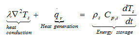
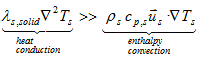
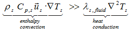
As the chemicals stored in containers can be solids or liquids, we must extend the heat conduction equation to allow considering in certain cases the motion of the fluid. After some restrictive assumptions, we obtain the following heat balance equation:
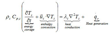
where λ, ρ, Cp, T, u, qr mean: thermal conductivity, density, specific heat, temperature, fluid with a velocity field us(x,y,z) and heat generated per unit volume during the decomposition reaction
![]()
with dα/dt the rate of the decomposition reaction expressed by the Arrhenius type equation as those applied in differential isconversional kinetics analysis and ΔTad the adiabatic temperature rise expressed by the heat of reaction ΔHr and the specific heat Cp,s : ΔTad = (-Δ Hr)/ Cp,s The heat balance equation is the same as for a solid body, except for the enthalpy transport, or convection term ![]()
To perform the exact heat balance the numerical techniques like finite element analysis, finite differences or finite volumes are generally applied. The sample is virtually divided into the set of adjoining elements (see Fig. 11). These elements are organized in a virtual mesh in which the rate of heat evolution is described by the advanced thermokinetics in each node of time and space.
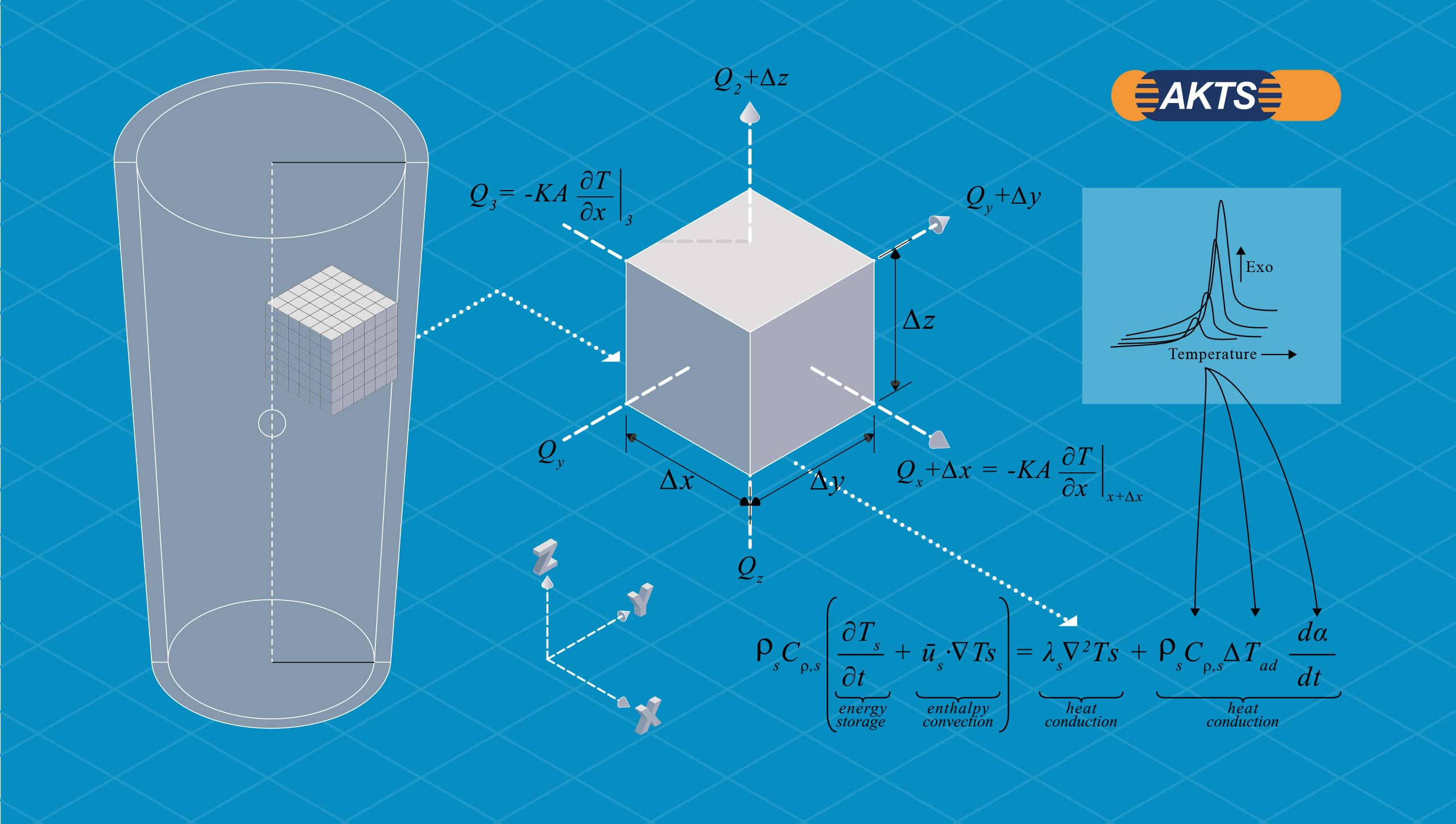
Fig. 11 – Generalized heat balance of a container and a volume element.
(A) Kinetic parameters calculated from DSC measurements, independent of the sample mass, enable the determination of the reaction rate required for the heat balance (inset). (B) Heat balance depends on the sample mass and has to be calculated by numerical techniques
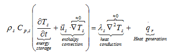
Heat balance in transient heat conduction (distributed) systems (for e.g. SOLIDS in containers)
If the examined substance is a SOLID, the main resistance to the heat transfer lies in the bulk of the substance because in solid materials the heat transfer occurs mainly by heat conduction and not by convection:
because ![]() = 0
= 0
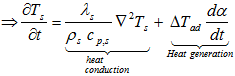
![]()
The thermal conductivity can be defined as the rate of heat transfer through a unit thickness per unit area per unit temperature difference, or, as the transport of energy due to random molecular motion across a temperature gradient.
Thermal conductivity depends mainly on the medium’s phase, temperature, density and molecular bonding within a solid structure. It means that in case of solids (and only in that case) there is a relevant temperature gradient ‘within’ the material from the center to the container wall.
In Cartesian (rectangular) coordinates, this temperature is expressed as T = T(x, y, z, t), where (x, y, z) indicate the variation of T gradient in the x-, y-, and z- axis directions, and t indicates its variation with time. We can write after some simplifications
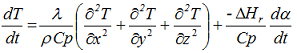
where λ is the thermal conductivity. For the analysis of limited cylinders with given H/D ratios (H: height, D: diameter) and flat lids (e.g. drums, containers, etc.), the cylindrical coordinates are generally used and the above equation can be written as
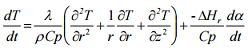
where r represents the radius of the cylinder and height is measured along the vertical z axis. Both above equations consider the variation of temperature with time as well as position in multidimensional systems. Further simplifications of these equations are possible if we consider the variation of temperature with time as well as position for one-dimensional heat conduction problems. In such cases, these equations can be simplified to
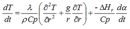
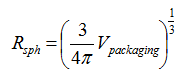
in which g is a geometry factor (g = 0 for an infinite plate, g = 1 for an infinite cylinder and g = 2 for a sphere). In this equation, the radius of the sphere with the same volume V as the considered packaging (so-called volume equivalent sphere) can be used. We have:
Heat balance in lumped systems (for e.g. LIQUIDS in containers)
For LIQUIDS with low viscosity
For liquids with low viscosity we have
![]()
The temperature of a material varies with time but remains uniform throughout at any time, T = T(t) according to Newton’s law of cooling. After some simplifications, the rate of the sample temperature change in classical lumped systems can be more generally expressed, as following :
where Cp, ρ, U, S, V, Φ, -ΔHr, dα/dt mean: specific heat capacity, density, overall heat transfer coefficient, surface, volume, thermal inertia, specific heat of reaction and reaction rate, respectively.
For lumped systems, the surface-to-volume ratio S/V can be used for the characterization of any sample container, regardless of its specific shape. The thermal inertia term (characterized by the Φ-factor) describes the heat loss and is given by
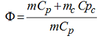
with m and mc representing the masses of the sample and the package (container), respectively. For large packages, if the lumped system assumption applies, the Φ-factor can be reasonably set to unity (Φ = 1) because the mass mc of the package is negligible compared to the sample mass mc. For smaller vessels, the Φ-factor, being generally larger than one, has a direct influence on the experimental adiabatic temperature rise ΔTad=-ΔHr/(Cp Φ).
For LIQUIDS with high viscosity
In case of LIQUIDS, heat is transferred not only by conduction but mainly by convection. Convection is the mode of heat transfer between the solid surface and the adjacent liquid (or gas) that is in motion, and it involves the combined effects of conduction and fluid motion. The concept of the Nusselt number (Nu) is generally used to determine the heat transfer coefficient h. The dimensionless Nusselt number represents the enhancement of heat transfer through a fluid layer as a result of convection relative to conduction across the same fluid layer. The larger the Nusselt number the more effective the convection.
It is defined and calculated as
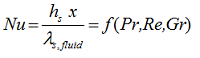
where x is the position along the interface in the direction of fluid flow. The Reynolds number (Re), Prandtl number (Pr) and Grashof number (Gr) are dimensionless terms which depend on the fluid velocity and on its physical properties such density, viscosity and expansion volume. Convection is classified as natural (or free) and forced convection, depending on how the fluid motion is initiated. In natural convection, any fluid motion is caused by natural means such as the buoyancy effect, which manifests itself as the rise of warmer fluid and the fall of the cooler fluid. In forced convection the fluid is forced to flow over a surface or in a pipe by external means such as a pump or a fan and the Grashof number
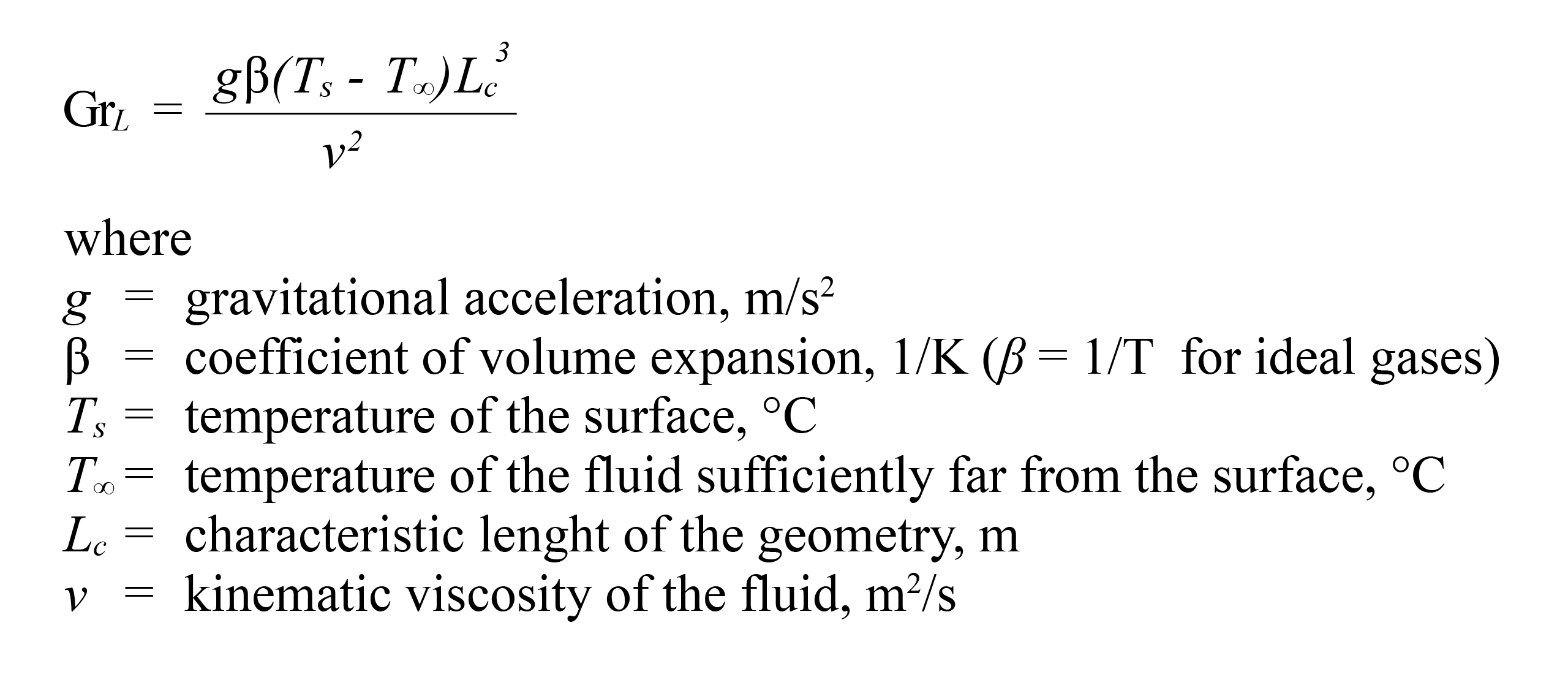
is generally used to approximate the ratio of the buoyancy force to the viscous force acting on a fluid. However, for mixtures in which the chemical reactions take place, physical properties such as volume coefficient of expansion or viscosity are usually unknown. Therefore, because heat is transferred mainly by convection the following simplifications can be made:
or
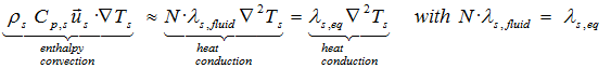
where the size of N increases with lower viscosity.
It comes for above that for liquids with high viscosity the energy equation leads to
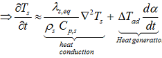
![]()
Boundary conditions
Beside some simplifications introduced into the above equations and because heat passes through the package into or out of the material, from or to the surroundings three kinds of time-dependent boundary conditions are generally applied: (i) prescribed temperature at the surface (Dirichlet condition), (ii) heat flux at the surface (Neumann condition) and (iii) heat transfer at the surface (Newton law, convective heat transfer or mixed boundary conditions). For heat transfer at the surface, another frequently applied simplification considers the rate of heat conduction through the wall of the package by using the overall heat transfer coefficient U, together with the thermal resistance concept R which is expressed by the equation

with
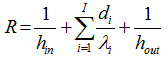
where di represents the thickness and λi the thermal conductivity of layer i in a multilayer package with I layers constituting the wall, and h the coefficient of heat transfer by convection inside the package (hin) in case of liquid samples and at the wall surface of the package (hout). The adiabatic conditions can be achieved by setting U=0. The appropriate boundary conditions together with the heat balance equations allow the self-heating of exothermally decomposed materials to be simulated after introducing the kinetic expression of the reaction rate dα/dt.
Heat balance equations applied for SADT for liquids and solids
Because some materials can decompose in solid or liquid (after melting) state and due to the fact that we have two different types of temperature distributions within the sample (with T uniform or with T gradients), four main different cases are conceivable during SADT evaluation. They are schematically presented in the Table.
Heat balance type | |||
|---|---|---|---|
| Distributed system with Tgradients (Solids) | Lumped system with T uniform (Liquids) | ||
| Physical state | Solid | S & S | S & L |
| Liquid | L & S | L & L |
|
Table 3 – Heat balance equations for liquids and solids considered during SADT evaluation.
- Case ‘L & L’: In this scenario, one applies the heat balance which is correct only for the liquid state and kinetic parameters evaluated from e.g. non-isothermal DSC data collected during the decomposition in the liquid state, i.e. above the melting point.
- Case ‘L & S’: The situation ‘L & S’ corresponds to the determination of the hazard properties using the kinetic parameters calculated from the decomposition in the liquid state (above the melting temperature) together with the heat balance approach valid for the solid state. Such an incorrect procedure leads to improper SADT value. The application of kinetic parameters characterizing decomposition in the liquid phase for the simulation of the thermal properties in the solid phase may be risky despite the application of the correct heat balance equations.
- Case ‘S & L’: This case illustrates the situation in which the inappropriate heat balance equation is applied. In large solid samples the temperature distribution is not even close to being uniform. The heat balance applicable for classical lumped systems valid for liquids only, cannot be used instead of the heat balance of the distributed system which has to be applied for the simulation of the thermal properties of large sample in the solid state. Mathematically, this approximation is used to simplify otherwise complex differential heat equations. However, in the case of solids, the correctness of application of the equation for liquids instead of those for solids depends in practice on the ratio of the internal and external heat flow resistances driven by the type of material and its surface area (packaging in the case of SADT), respectively. This ratio can be estimated from the Biot-number which indicates if the assumption concerning the “object temperature” at any given time assuming no spatial temperature variation within the object may be acceptable.
- Case ‘S & S’: For the prediction of the hazard properties of solids that decompose already at temperatures below their melting point, the correct procedure for the prediction of their SADT temperature consists in applying both, the kinetic parameters and heat balance characteristics for the solid state. As far as the DSC technique is concerned, the experiments for such materials should be collected isothermally in a narrow temperature window below the melting point.
As a general rule, the correct procedure for the prediction of the thermal behavior of any material consists in applying correctly both, the kinetic parameters and heat balance depending on the material state.
The kinetic based approach for the determination of Self Accelerating Decomposition Temperature (SADT)
Because in the strict sense the mechanisms of the decompositions are not fully known our simulations presented below are based on the kinetic parameters evaluated by the differential isoconversional kinetic analysis which does not require any knowledge of the decomposition mechanism. The value of a heat transfer coefficient U in the first approximation was based on the UN recommendations [41] and the claims found in the paper published by BAM [42] in which in the large scale experiments the U value is considered in the range between 4-8 W m-2 K-1.
The Self-Accelerating Decomposition Temperature (SADT) is an important parameter that characterizes thermal hazard possibility under transport conditions of self-reactive substances. SADT is used in international transportation regulations and is referenced in the United Nations presented in ”Recommendations on the Transport of Dangerous Goods, Manual of Tests and Criteria” (TDG) [41]. Globally Harmonized System (GHS) has inherited SADT as a classification criterion for self-reactive substances. According to the Recommendations on TDG, SADT is defined as ”the lowest temperature at which self-accelerating decomposition may occur with a substance in the packaging as used in transport”. An important feature of SADT is that it is not an intrinsic property of a substance but a measure of combined effect of ambient temperature, decomposition kinetics, packaging size and heat transfer properties of the substance and its packaging.
The Manual of Tests and Criteria of the United Nations regarding transport of dangerous goods and on the globally harmonized system of classification and labeling of chemicals indicates that the characterization of materials is based on heat accumulation storage tests.
The regulatory compliance definitions are:
- SADT is the lowest environment temperature at which overheat in the middle of the specific commercial packaging exceeds 6°C(ΔT6) after a lapse of a seven day period (168 hours) or less. This period is measured from the time when the packaging center temperature reaches 2°C below the surrounding temperature.
- SADT is the critical ambient temperature rounded to the next higher multiple of 5°C.
The first definition is based on two essential parameters: maximal permissible overheating temperature and minimal acceptable induction period. The second definition considers only one parameter: the critical ambient temperature of thermal runaway rounded to the next higher multiple of 5°C without introducing any fixed transportation time into the definition.
Bearing in mind the abovementioned SADT definitions, several additional factors have to be considered for the proper determination of SADT :
- The intrinsic properties of the test material such as, kinetic parameters of decomposition (activation energy, pre-exponential factor in the Arrhenius equation) and physico-chemical properties such as thermal conductivity, specific heat and density.
- The external properties of the sample that can be changed arbitrarily, e.g. sample mass, geometry and physical properties of the sample holder/container.
From the above factors, especially the thermal conductivity (in case of solid or high viscous substances), the heat transfer coefficient and sample mass may influence the calculation of SADT in a significant way. As thermal conductivities of chemicals are not always exactly known and as both, container volume and sample mass, can be arbitrarily changed, their influence on SADT was examined in broad range of their changes. Simulations have been done for:
- Sample holders shaped as cylinders with internal volumes of: 5, 10, 25, 50, 100, 250 and 500 L.
- Following equivalent thermal conductivities λs,eq : 0.1 and 1W m-1K-1.
Illustration of choice of possible parameters regarding container materials and chemical substance for SADT calculations can be found in Fig.12.
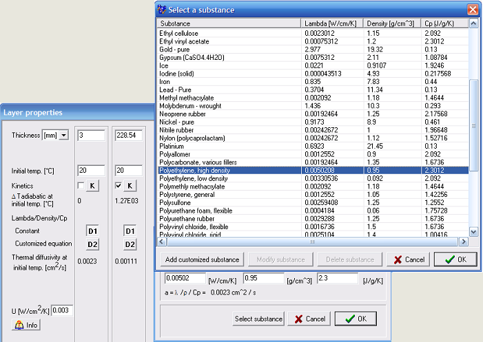
Fig. 12 – Parameters regarding container materials and chemical substance for SADT calculations.
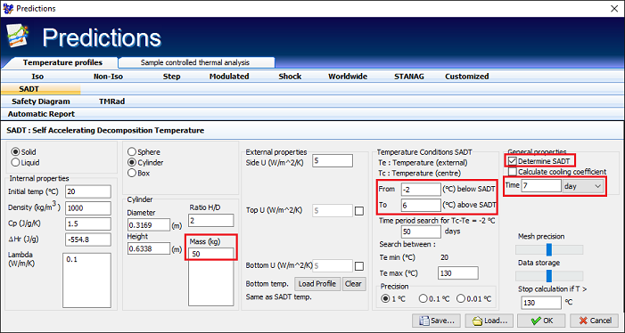
Fig. 13 – The input of parameters in Thermal Safety Software required for SADT evaluation
| Density ρ | 1000 kg/m3 |
| Specific heat Cp | 1.5 Jg/K |
| Thermal conductivity λ | 0.1 W/(m K) < λeq < 1 W/(m K) (through numerical variations) |
| Sample holder | Drum (Height/Diameter =2) (5 L < sample holder volume < 500 L) |
| Heat of reaction ΔHr | -554.8 J/g (measured from DSC) |
| Heat transfer coefficient U | 5 W/(m2 K) |
Table 4 – Specification of the properties of the substance and the system applied during simulation of SADT
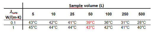
Table 5 – Dependence of SADT (°C) on thermal conductivity λs,eq and amount of substance expressed by the sample volume (L) in drums with H/D = 2.
Table 5 presents the results of the SADT simulation for λs,eq values 0.1 and 1 W/(m K) and sample volumes between 5 and 500 L. The simulations were done for cylinders with the ratio H/D = 2 with flat lids. The results in table 5 clearly shows that both, thermal conductivity and sample volume influences the SADT values. For a 50 L drum corresponding to the H.1-test (filling height H = 63.4 cm and D = 31.7 cm), SADT with an assumed thermal conductivity λ of 0.1 W/(m K) amounts to 39°C (see Tab. 5. and Fig. 15.) whereas under assumption of larger heat transfer for an ”apparent” conductivity term λs,eq = 1 W/(m K) SADT amount to about 43°C respectively (see Table 5).
SADT is therefore influenced by the rate of heat formation and its amount (heat of the reaction and its mechanism as decelerating or autocatalytic type) and the rate of heat transfer from the system which is mainly dependent on the thermal conductivity and sample volume.
Fig. 14 presents the surrounding temperature corresponding to SADT and the evolution of the temperature inside the drum at its center (R=0;H/2). The average reaction progress αvs. time is presented at the bottom of Fig. 14.
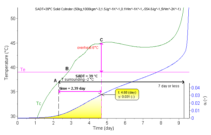
Fig. 14 – Simulation of the SADT for 50 kg of the material in a drum with filling height H = 63.4 cm and D = 31.7 cm (the other parameters are given in Tab. 4.) (pink: surrounding temperature Te, green: sample temperature in the center of the drum Tc , blue: reaction extent α).
Our simulations based on kinetic parameters evaluated from DSC signals and the correct heat balance in the system indicate that a temperature of 39°C is the lowest environment temperature at which overheat in the middle of considered 50-kg packaging exceeds 6°C (ΔT6) after a lapse of seven days (168 hours) or less. This period is measured from the time when the packaging centre temperature reaches 2°C below the surrounding temperature (after ca. 2.3 days) (Point A). After about 2.8 days (Point B) the centre temperature is equal to the surrounding temperature. The overheat of 6°C occurs after about 4.7 days (Point C). At this time the average reaction progress in the 50 kg package amounts to 0.031 (ca. 3.1%) (bottom, right axis). Fig. 15 presents the calculated spatial distribution of the temperatures (left column) and reaction progresses (right column) in the drum after lapse of time represented by the points A, B and C i.e. when the center temperature differs by -2°C, 0 and +6°C, respectively compared to the surrounding temperature.
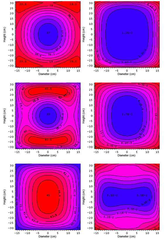
Fig. 15 – Simulations of the spatial distribution of temperature (left) and reaction progress α (right) for a mass of 50 kg in a drum with ratio H/D = 2 after periods of time represented by the points A (top), B (middle) and C (bottom) depicted in Fig. 14.
Conclusion
The evaluation of SADT based on DSC experiments and precise heat balance of the system has several advantages:
- It is fast: Reliable screening of candidate materials by revelation of potentially unstable mixtures at prolonged times and temperature exposures can be done within few hours.
- It is economical: The determination of the kinetics offers very significant time/expertise savings compared to real time analysis which can extend over prolonged periods, even months.
- It is convenient: DSC devices are widely available and require a small amount of material only.
- It is versatile: With one set of measurements different scenarios can be simulated.
References
[1] AKTS SA, https://www.akts.com (AKTS-Thermokinetics software).
[2] M.E. Brown et al. Computational aspects of kinetic analysis. The ICTAC Kinetics project data, methods and results. Thermochim. Acta, 355 (2000) 125.
[3] M. Maciejewski, Computational aspects of kinetic analysis. The ICTAC Kinetics Project – The decomposition kinetics of calcium carbonate revisited, or some tips on survival in the kinetic minefield. Thermochim. Acta, 355 (2000) 145.
[4] A. Burnham, Computational aspects of kinetic analysis. The ICTAC Kinetics Project – multi-thermal-history model-fitting methods and their relation to isoconversional methods. Thermochim. Acta, 355 (2000) 165.
[5] B. Roduit, Computational aspects of kinetic analysis. The ICTAC Kinetics Project – numerical techniques and kinetics of solid state processes. Thermochim. Acta, 355 (2000) 171.
[6] S. Vyazovkin, A.K. Burnham, J.M. Criado, L.A. Pérez-Maqueda, C. Popescu, N. Sbirrazzuoli, ICTAC Kinetics Committee recommendations for performing kinetic computations on thermal analysis data, Thermochim. Acta, 520 (2011) 1-19.
[7] S. Vyazovkin, K. Chrissafis, M.L. Di Lorenzo, N. Koga, M. Pijolat, B. Roduit, N. Sbirrazzuoli, J.J. Suñol, ICTAC Kinetic Committee recommendations for collecting experimental thermal analysis data for kinetic computations, Thermochim. Acta, 590 (2014) 1-23.
[8] B. Roduit, W. Dermaut, A. Lunghi, P. Folly, B. Berger and A. Sarbach, J. Therm. Anal. Cal., 93 (2008) 1, 163-173.
[9] B. Roduit, P. Folly, B. Berger, J. Mathieu, A. Sarbach, H. Andres, M. Ramin and B. Vogelsanger, J. Therm. Anal. Cal., 93 (2008) 1, 153-161.
[10] B. Roduit, L. Xia, P. Folly, B. Berger, J. Mathieu, A. Sarbach, H. Andres, M. Ramin, B. Vogelsanger, D. Spitzer, H. Moulard and D. Dilhan, J. Therm. Anal. Cal., 93 (2008) 1, 143-152.
[11] B. Roduit, M. Hartmann, P. Folly, A. Sarbach, P. Brodard, R. Baltensperger, J. Therm. Anal. Calorim., 117 (2014) 1017-1026.
[12] B. Roduit, M. Hartmann, P. Folly, A. Sarbach, P. Brodard, R. Baltensperger, Thermochim. Acta, 621 (2015) 6-24.
[13] B. Roduit, M. Hartmann, P. Folly, A. Sarbach, R. Baltensperger, Thermochim. Acta, 579 (2014) 31-39.
[14] B. Roduit, Ch. Borgeat, B. Berger, P. Folly, B. Alonso, J.N. Aebischer and F. Stoessel, J. Therm. Anal. Cal., ICTAC special issue, 80 (2005) 229-236.
[15] B. Roduit, Ch. Borgeat, B. Berger, P. Folly, B. Alonso, J.N. Aebischer, J. Therm. Anal. Cal., ICTAC special issue, 80 (2005) 91-102.
[16] P. Folly, Chimia, 58 (2004), 394.
[17] M. Dellavedova, C. Pasturenzi, L. Gigante, A. Lunghi, Chem. Eng. Trans., Vol.26 (2012) 585-590.
[18] Hemminger W. F., Sarge, S. M., J. Therm. Anal., 37 (1991), 1455.
[19] P. Budrugeac, J. Therm. Anal., 68 (2002) 131.
[20] H. L. Friedman, J. Polym. Sci, Part C, Polymer Symposium (6PC), 183 (1964).
[21] T. Ozawa: Bull. Chem. Soc. Japan, 38 (1965) 1881.
[22] J.H. Flynn, L.A. Wall, J. Res. Nat. Bur. Standards, 70A (1966), 487.
[23] U. Ticmanis, G. Pantel, S. Wilker, M. Kaiser, Precision required for parameters in thermal safety simulations, 32nd International Annual Conference of ICT July, (2001), 135.
[24] D.I. Townsend, J.C. Tou, Thermal hazard evaluation by an accelerating rate calorimeter, Thermochim. Acta 37 (1980) 1–30.
[25] F. Stoessel, J. Steinbach, A. Eberz: Plant and process safety, exothermic and pressure inducing chemical reactions, In: Ullmann’s encyclopedia of industrial chemistry. Weise E (Eds), VCH, Weinheim (1995):343-354.
[26] A. Keller, D. Stark, H. Fierz, E. Heinzle, K. Hungerbuehler: Estimation of the TMR using dynamic DSC experiments. Journal of Loss Prevention in the Process Industries (1997) 10(1):31-41.
[27] N.N. Semenov, Prog. Phys. Sci. U.S.S.R., 23 (1940) 251-292; National advisory committee for aeronautics, Technical memorandum, 1024 Washington (1942) 1-57.
[28] D.A. Frank-Kamenetskii, 2nd Ed., Translated from Russian by J.P. Appleton, Plenum Press, New York-London (1969) 375.
[29] J.M. Dien, H. Fierz, F. Stoessel, G. Killé: The thermal risk of autocatalytic decompositions: a kinetic study. Chimia (1994) 48(12):542-550.
[30] D.W. Smith, Assessing the hazards of runaway reactions, Chem. Eng., 14, (1984) 54.
[31] T. Grewer, Thermochim. Acta, 225 (1993) 165.
[32] R. Gygax, International Symposium on Runaway reactions, March 7-9, 1989, Cambridge, Massachusetts, USA, 52.
[33] F. Stoessel, Design thermally safe semibatch reactors, Chem. Eng. Prog., (1995) September 46-53.
[34] F. Stoessel, Applications of reaction calorimetry in chemical engineering, J. Therm. Anal., 49 (1997) 1677-1688.
[35] F. Stoessel, Safety issues in scale-up of chemical processes. Current Opinion in Drug Discovery & Development (2001) 4(6): 834-838.
[36] F. Stoessel, Sécurité thermique des procédés, Evaluation des risques d’emballement. Vol. SE5010. 2013, Paris: Techniques de l’ingénieur.
[37] F. Stoessel, Méthodes thermiques en sécurité des procédés chimiques. Techniques de l’Ingénieur, (2018) p1312 (ref. article : p1312). Publications des résultats de thèses.
[38] F. Stoessel, Thermal Safety of Chemical Processes, Risk Assessment and Process Design, 2. Auflage – März 2020, WILEY-VCH Verlag GmbH & Co. CGaA.
[39] A heat transfer textbook Third Edition, John H. Lienhard IV / John H. Lienhard V, Phlogiston Press, Cambridge Massachusetts, 2008.
[40] H. Fierz, J. Hazard. Mater., A96 (2003) 121-126.
[41] UN Recommendations on the Transport of Dangerous Goods, Manual of Tests and Criteria, 5th revised edition. United Nations, New York and Geneva, (2009) 297-316.
[42] M. Steensma, P. Schuurman, M. Malow, U. Krause, K.D. Wehrstedt, J. Hazard. Mater., A117 (2005) 89-102.
[43] B. Roduit, M. Hartmann, P. Folly, A. Sarbach, P. Brodard, R. Baltensperger, Chem. Eng. Trans., VOL. 48 (2016).
[44] B. Roduit, M. Hartmann, P. Folly, A. Sarbach, A, Dejeaifve, R. Dobson, K. Kurko, Thermochim. Acta, 665 (2018) 119-126.